Questions
- Does an array of sonar transducers separated by hundreds of metres or kilometres give sensitivity advantages over conventional towed arrays for detecting surface ships and submarines?
- How do vertically suspended arrays compare with towed arrays?
- If each distributed node is itself a vertical array, does that offer desirable traits?
Approach. Published measurements and systems (notebook 01) combined with simulations built for this study: array gain with ocean coherence limits and directional noise, sonar-equation coverage maps, focused-beamforming and time-of-arrival localisation, normal-mode depth discrimination, and finite-difference time-domain (FDTD) wave simulations across a thermocline (notebooks 02–05). Node positions and clocks are assumed known, as the brief allows; the conclusions concern physics, not engineering or cost.
Answers in brief
Q1 · Widely spaced nodes versus a towed array
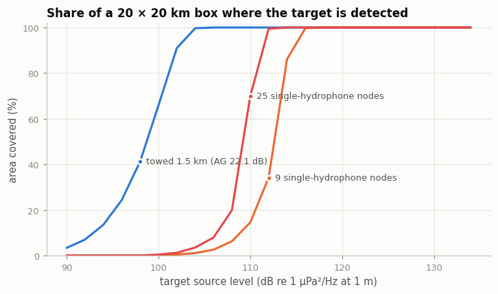
Not for sensitivity: spacing itself buys no gain. Array gain against noise comes from the number of sensors whose signals add coherently. Ocean signals stay coherent over only ~20–40 wavelengths in shallow water (≈100–200 m at 300 Hz), so nodes hundreds of metres to kilometres apart cannot be added coherently across most of the passive band. Their outputs can only be fused incoherently, worth about 5 log₁₀ M dB for a steady signal. In the coverage model (150 m shelf, 300 Hz), nine single-hydrophone nodes need a target ~14 dB louder than a 1.5 km towed array needs to cover the same 20 × 20 km box, despite being closer to it.
Wide spacing wins on localisation: a position fix from one event (when 3–4 nodes hear it), with no left/right ambiguity. It also brings freedom from tow-platform noise, diversity against fading and target aspect, and the choice of where to put sensors. A coherent sum across 5 km-spaced nodes beats plain incoherent fusion only below ~8–30 Hz, depending on the coherence length.
Q2 · Vertical versus towed arrays
A vertical array trades bearing for depth; whether it has more gain depends on the water. For equal element counts (32 elements, 300 Hz):
| Noise field | Vertical array | Towed (horizontal) array |
|---|---|---|
| Deep water, wind noise dominates (plane-wave upper bound) | 23 dB | 14 dB |
| Deep water, distant shipping dominates | 7.5 dB | 16 dB |
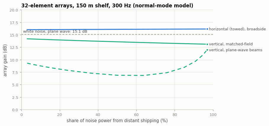
| 150 m shelf, any mix: matched-field / plane-wave beams | 13–14 / 7–12 dB | 16 dB |
On a shelf the target's signal is spread over many modes and wind noise fills the deep-water notch, so the horizontal array has more gain. The vertical array's advantages are information: it spans the thermocline (a fixed-depth array gains or loses 1–2 dB relative to the column average depending on the side of the layer the target is), and it can tell a surface ship from a submarine by estimating source depth, which a broadside towed array cannot. It gives no bearing on its own, and it does not move.
Q3 · A network of vertical arrays
Yes: roughly towed-array sensitivity, plus 3D position and classification.
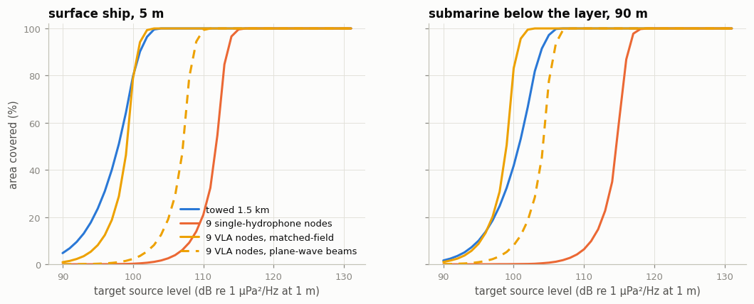
- Sensitivity: on a shelf each node brings ~6–14 dB of array gain and the network adds proximity. 9 VLA nodes with matched-field processing cover the box against the same targets as the 1.5 km towed array (~101 dB for a surface ship) and ~3 dB quieter ones when the target is below the layer. That is an upper bound (known environment and range, no vertical-coherence loss); with conventional beams they need targets ~2–8 dB louder. Real tow self-noise (3–6 dB) moves the balance towards the network.
- Localisation: horizontal position from the network geometry, and depth and range from each node.
- Classification: 92–100% correct surface/submerged calls from about −10 dB SNR per hydrophone in the model.
The ocean still forbids coherent gain between nodes at normal passive frequencies. The case for the concept rests on what it adds at equal sensitivity; the open questions are engineering ones: moorings, power, communications and suspension noise.
What drives the answers (notebook 06)
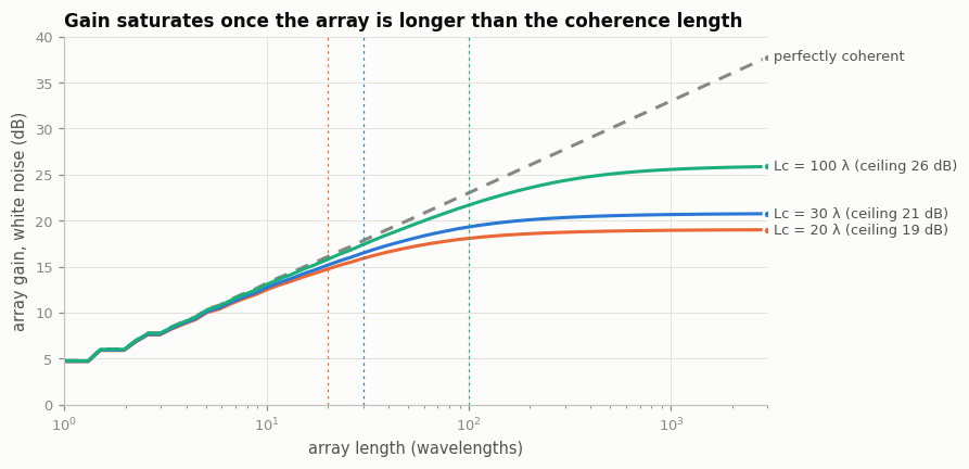
- Coherence caps array gain at about 10 log₁₀(4 L_c/λ): ~21 dB for L_c = 30 λ, ~26 dB for 100 λ. Longer arrays buy resolution, not sensitivity.
- Frequency: small (hull) apertures are pushed up in frequency until absorption and bottom loss stop them (a 5 m bow array: a few kHz); long apertures are capped by coherence and want low frequency.
- The thermocline is large in deep water at mid frequency: a submarine below a 60 m layer is ~9–12 dB (1 kHz) to ~26–34 dB (3.5 kHz) harder for a hull sonar in the layer to hear than a surface source. It is transparent at 100 Hz and only ~5–7 dB on a 150 m shelf, where the seabed refills the column.
A 10-USV formation at 100 Hz (notebook 07)
Ten USVs with one hydrophone each at λ/2 make a 70 m array: ~11 dB, about 10 dB short of a 1.5 km towed array. Giving each USV a dipped 20-hydrophone vertical line (200 hydrophones) brings it within 3–4 dB with matched-field processing, and ahead by 3–5 dB only if the vehicles and lines are much quieter than the tow. The requirements are hydrophone count, quietness, an environment model, and ~1 m knowledge of every hydrophone including line tilt.
Key figures
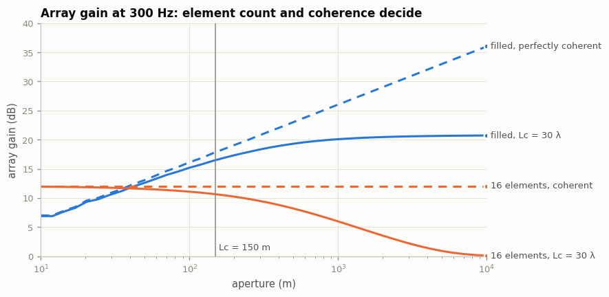
Array gain is set by coherent element count, not aperture (notebook 02)
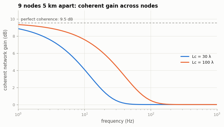
Coherent gain across nodes 5 km apart vanishes above a few tens of Hz (notebook 02)
Coverage against quiet targets: towed array, single-hydrophone nodes and VLA nodes (notebooks 02 and 04)
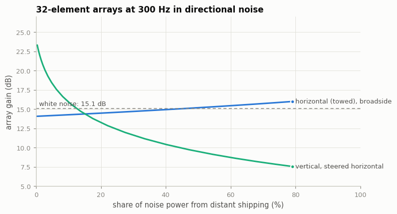
Horizontal versus vertical array gain: deep-water picture, then a shallow shelf (notebook 03)
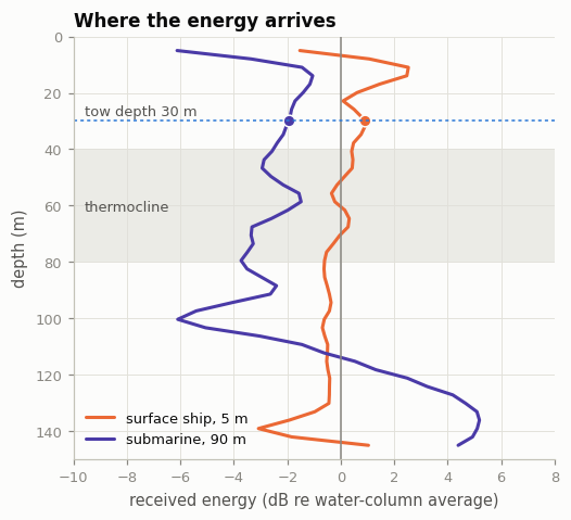
Where the energy arrives: surface ship versus submarine below the layer (notebook 03, from FDTD)
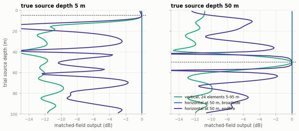
Only the vertical array (or an endfire towed array) sees source depth (notebook 03)
Pre-rendered animations
| Case | Shows | Notebook |
|---|---|---|
plan_towed |
a towed array localises to a bearing band plus its left/right mirror | 02, 05 |
plan_distributed |
9 coherent nodes 5 km apart focus to a half-wavelength spot | 02, 05 |
plan_distributed_jitter |
the same nodes with ~0.4 λ path errors: the coherent focus breaks up | 02, 05 |
section_surface_ship |
FDTD, 150 m shelf with thermocline: surface source heard by a vertical array | 03, 05 |
section_sub_below_layer |
FDTD, source below the layer: energy deep; tow depth 7 dB below the best depth | 03, 05 |
plan_usv_line |
10 USVs at λ/2 (100 Hz): a broad bearing fan and its mirror | 07 |
plan_usv_ring |
10 USVs on a 190 m ring: a tight spot, no mirror | 07 |
pe_* |
parabolic-equation TL maps: deep water and shelf, 100 Hz / 1 kHz / 3.5 kHz, ship and submarine | 06 |
Every case is a set of named parameters in sonarsim/cases.py; notebook 05 shows how to change them and render your
own.
Assumptions and limits
- Coherence is modelled as exponential decorrelation with length $L_c$ (20–100 λ swept; 30 λ default, from Carey's shallow-water measurements). Real coherence varies with internal waves, range and path.
- Propagation for coverage is range-only: spherical to the water depth, cylindrical beyond, with absorption and 0.5 dB/km bottom loss. Depth structure (the layer) is applied from two FDTD cases at 100 Hz, not a general law.
- Noise is modelled, not measured: a free-field directional model (wind from above, shipping near horizontal) for the deep-water picture, and Kuperman–Ingenito normal-mode noise in a Pekeris waveguide for the shelf.
- Vertical-array gain on the shelf assumes perfect vertical coherence of the modal field; matched-field figures assume the environment is known. Real mismatch lowers both.
- Detection uses a steady signal, $P_d \approx 0.6$, $P_{fa} = 10^{-4}$, no fading, no tow self-noise, and conventional (not adaptive) beamforming. All coverage is on a 150 m shelf at 300 Hz; deep-water, low-frequency surveillance is outside the model.
- FDTD is 2D: sources are line sources and spreading is cylindrical, so absolute levels are not 3D levels. Depth structure, refraction and multipath are physical.
- Matched-field depth estimation uses a known Pekeris waveguide; real environmental uncertainty widens the peaks.
- Target source levels are swept (90–135 dB re 1 µPa²/Hz at 1 m), because real submarine levels are not public.
- Not modelled: cost, deployment, communications, power, platform motion and strumming, active sonar in detail.
Using this report
- Hosted: open the notebooks in the browser (JupyterLite). The code runs in your browser; heavy FDTD cases have
a
quick=Truepreview mode. - Locally:
pip install numpy scipy matplotlib pillow jupyterlab, thenjupyter labin this folder. ffmpeg enables MP4 output. - Regenerate everything:
python scripts/render_cases.py && python scripts/build_notebooks.py.
Sources
Carey (1998), The determination of signal coherence length based on signal coherence and gain measurements in deep and shallow water, JASA 104, 831 (link) and the Carey number review in Acoustics Today (pdf) · TB-16 (GlobalSecurity) · SURTASS (Wikipedia; GlobalSecurity) · SOSUS (DOSITS) · DARPA DASH / TRAPS (DARPA) · Noise directionality (Internoise 2014; Kuperman & Ingenito 1980) · VLA depth discrimination (JASA EL 2016); HLA mode-subspace depth discrimination (JASA 2013) · Reliable acoustic path (JASA 2009) · Random arrays (Lo 1964) · Towed-array left/right ambiguity (Kaouri) · Multistatic sonar (Fewell & Ozols; multistatic sonobuoy fields) · Textbooks: Urick, Principles of Underwater Sound (1983); Jensen, Kuperman, Porter & Schmidt, Computational Ocean Acoustics (2011); Albersheim (1981), IEEE Trans. AES 17, 131.
01 · Background: arrays, coherence and the sonar equation
This notebook sets out the physics and the published facts the rest of the study relies on. The later notebooks (02–04) answer the three questions with simulations; the summary is in 00_summary.
Scope. Passive detection of surface ships and submarines by the sound they radiate, mainly at 10 Hz–1 kHz, where machinery tonals and broadband cavitation noise propagate furthest. Nodes are assumed to know their positions and share synchronised clocks, as the brief allows. Active (echo-ranging) operation is touched on where it changes a conclusion.
1. The passive sonar equation
A detection needs the signal after processing to exceed a threshold:
$$\mathrm{SNR} = SL - TL - (NL - AG) \;\geq\; DT$$
| Term | Meaning | Typical control |
|---|---|---|
| $SL$ | source level of the target (dB re 1 µPa²/Hz at 1 m) | the target |
| $TL$ | transmission loss from target to sensor | geometry, propagation, how close the sensor is |
| $NL$ | ambient + self noise at the sensor | sea state, shipping, platform self-noise, sensor depth |
| $AG$ | array gain: SNR improvement of the array over one hydrophone | number of coherent elements, noise directionality |
| $DT$ | detection threshold for the wanted $P_d$, $P_{fa}$, bandwidth, integration time | processing |
Every design question in this study moves one of these terms. A wide sensor spacing does not change $AG$ by itself; it changes $TL$ (sensors nearer the target), the geometry available for localisation, and what can be combined coherently. The notebooks keep these effects separate.
2. Array gain and why it depends on coherence
For $N$ hydrophones whose signals add in phase while their noises are independent, delay-and-sum beamforming gives
$$AG = 10\log_{10} N .$$
Two conditions hide in that formula:
- The noise must be uncorrelated between elements. In isotropic noise this holds for spacing $\geq \lambda/2$; in directional noise (wind noise from above, shipping near the horizontal) the array shape decides how much noise it rejects. This is where vertical and horizontal arrays differ (notebook 03).
- The signal must stay coherent across the array. The ocean scrambles the phase of a signal over distance (internal waves, multipath, fluctuating paths). The signal coherence length $L_c$ is the separation over which coherence is lost. Beyond it, extra aperture adds noise and signal equally and the gain saturates.
Measured coherence lengths. Carey (1998) combined coherence and array-gain measurements and found horizontal coherence lengths in shallow water of about 20–40 wavelengths, averaging 30 λ, now called the "Carey number" (Acoustics Today review; Carey 1998, JASA 104, 831). The SW06 experiment at 200 Hz found the same 20–40 λ range, falling sharply while non-linear internal-wave trains crossed the path. Deep-water paths are generally more coherent, but by how much varies with range, frequency and path; the simulations therefore sweep $L_c$ instead of assuming one value.
In metres, 30 λ is small at the frequencies most passive sonars use:
Code
import sys, os
sys.path.insert(0, os.path.abspath('..'))
import numpy, scipy, matplotlib, PIL  # named here so the in-browser (JupyterLite) kernel loads them
import numpy as np
import matplotlib.pyplot as plt
from sonarsim import style, physics
style.use()

f = np.logspace(0.7, 3.3, 200)          # 5 Hz ... 2 kHz
lam = 1500 / f
fig, ax = plt.subplots(figsize=(7.2, 3.8))
for n, col, lab in [(20, style.MUTED, '20 λ'), (30, style.BLUE, '30 λ (Carey number)'), (100, style.ORANGE, '100 λ (optimistic, deep water)')]:
    ax.loglog(f, n * lam, color=col, lw=2)
    style.label_end(ax, f[-1], n * lam[-1], lab, col)
ax.axhspan(100, 10000, color=style.GRID, alpha=0.5, lw=0)
ax.text(250, 2500, 'typical distributed-node spacing\n(100 m – 10 km)', fontsize=8.5, color=style.INK2)
ax.set_xlabel('frequency (Hz)'); ax.set_ylabel('coherence length (m)')
ax.set_title('Signal coherence length in metres', loc='left')
ax.set_xlim(5, 2000); ax.set_ylim(1, 1e5)
style.save(fig, 'coherence_length_m')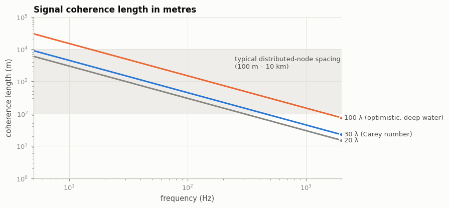
At 300 Hz, 30 λ is about 150 m; at 30 Hz it is 1.5 km. Nodes spaced hundreds of metres to kilometres apart are therefore mutually incoherent across most of the passive band. Only in the lowest band (roughly 5–30 Hz), and more so in deep water, can kilometre-scale spacings stay partly coherent. Notebook 02 turns this into gain numbers.
3. The reference systems
| System | Geometry | Published figures |
|---|---|---|
| Tactical fat-line towed array (TB-16 class) | horizontal line towed behind a ship or submarine | 73 m (240 ft) acoustic module, 3.5 in diameter, 730 m (2,400 ft) tow cable (GlobalSecurity) |
| Surveillance towed array (SURTASS) | long horizontal line from a slow ship | ~1,500 m array, towed at 150–460 m depth, minimum ~3 kt (SURTASS); the twin-line variant tows two lines 2.2–8.8 m apart to resolve the left/right ambiguity (GlobalSecurity) |
| Fixed bottom arrays (SOSUS) | horizontal lines on the seabed near the shelf edge, using the deep sound channel | first installation 1952: 1,000 ft line of 40 hydrophones at 1,440 ft depth (DOSITS) |
| Deep distributed nodes (DARPA DASH / TRAPS) | passive nodes on the deep seafloor looking up, exploiting the reliable acoustic path and the quiet deep ocean | (DARPA DASH) |
| SURTASS LFA source | vertical line of up to 18 projectors, centre ~120 m | a vertical array used for vertical directivity (SURTASS) |
Known towed-array limitations: a single line cannot tell which side a sound comes from (left/right ambiguity, e.g. Kaouri, Oxford thesis); it sits at one depth set by speed and cable scope; it hears its own tow platform and flow noise, worst towards the forward endfire; and its shape wanders when the ship turns, blurring the beams.
4. Ambient noise is directional
Wind and waves make noise at the surface; it arrives at a submerged sensor mainly from above, strongest near the vertical. Distant shipping arrives near the horizontal, because only low-angle paths survive long ranges. In downward-refracting water a noise notch forms near the horizontal (Internoise 2014 review; Kuperman & Ingenito 1980). The same review notes that vertical arrays steered horizontally gain much more than horizontal arrays in surface-dominated noise. Notebook 03 models this with a two-component directionality: wind noise $\propto \sin(\text{elevation})$ from above (dipole surface sources) with partial bottom reflection, plus a band of shipping noise near the horizontal.
Code
from sonarsim import arrays
el = np.linspace(-90, 90, 361)
fig, ax = plt.subplots(figsize=(7.2, 3.4))
for ship, col, lab in [(0.0, style.AQUA, 'wind only'), (1.0, style.ORANGE, 'wind + distant shipping')]:
    d = arrays.noise_directionality(el, wind=1.0, shipping=ship, bottom_reflection=0.3)
    ax.plot(el, 10*np.log10(d/d.max()), color=col)
    style.label_end(ax, 90, 10*np.log10(d[-1]/d.max()), lab, col)
ax.set_xlabel('arrival elevation (deg, + = from above)'); ax.set_ylabel('noise per solid angle (dB)')
ax.set_ylim(-20, 2); ax.set_xlim(-90, 90)
ax.set_title('Model noise directionality used in notebook 03', loc='left')
style.save(fig, 'noise_directionality')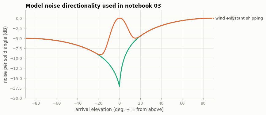
5. Vertical arrays and source depth
In a waveguide, the field from a source is a sum of normal modes whose shapes depend on depth. A vertical array samples those shapes directly, so it can estimate source depth by matched-field processing or mode filtering, which tells a surface ship from a submarine (Source depth discrimination with a vertical line array, JASA 2016). A horizontal array can do this only when it is long and the source is near endfire, using mode wavenumbers instead of mode shapes (mode subspace projections with an HLA, JASA 2013). Deep vertical arrays can also exploit the reliable acoustic path, a direct refracted path from near-surface sources to a deep receiver (Passive detection using the RAP, JASA 2009).
6. Sparse arrays
Elements spaced much more than λ/2 produce grating lobes: copies of the main beam in other directions. Randomising the positions spreads them into a sidelobe floor whose average power is about $1/N$ of the main lobe (Lo 1964). A network of 9 nodes therefore focuses with sidelobes averaging only about −10 dB even when perfectly coherent. Broadband processing helps: the grating lobes of different frequencies fall in different places and average out, which is why the animations use a broadband transient.
7. Combining incoherent sensors
When sensors cannot be combined coherently, their detector outputs can still be fused. For $M$ equal-SNR independent looks, the required per-look SNR falls by roughly $5\log_{10}M$ (Albersheim's equation gives 6.9 dB for $M = 9$ at $P_d=0.5$, $P_{fa}=10^{-4}$). The optimal weighted fusion used in the coverage maps adds deflections in quadrature, $\mathrm{SNR}_{\text{eff}} = \sqrt{\sum \mathrm{SNR}_i^2}$, the same $5\log_{10}M$ law for equal SNRs. Coherent combination would give $10\log_{10}M$, so incoherent fusion recovers only half the decibels. That holds for a steady signal; when the signal fades (multipath, aspect-dependent radiation) and a high $P_d$ is required, independent looks also bring diversity gain, which can be worth several dB more. Multistatic sonobuoy studies reach similar conclusions: the benefit of many receivers comes mainly from geometry and coverage, not per-receiver gain (Fewell & Ozols, DSTO; design of multistatic sonobuoy fields).
Code
M = np.arange(1, 65)
fig, ax = plt.subplots(figsize=(7.2, 3.6))
ax.plot(M, 10*np.log10(M), color=style.BLUE)
style.label_end(ax, M[-1], 10*np.log10(M[-1]), 'coherent: 10 log M', style.BLUE)
ax.plot(M, [physics.incoherent_gain_db(m) for m in M], color=style.ORANGE)
style.label_end(ax, M[-1], physics.incoherent_gain_db(M[-1]), 'incoherent (Albersheim)', style.ORANGE)
ax.plot(M, physics.fuse_snr_db(np.zeros((1, 1)))*0 + 5*np.log10(M), color=style.AQUA, ls=(0, (4, 3)))
style.label_end(ax, M[-1], 5*np.log10(M[-1]), '5 log M', style.AQUA)
ax.set_xlabel('number of sensors or nodes combined'); ax.set_ylabel('gain (dB)')
ax.set_xlim(1, 64); ax.set_ylim(0, 20)
ax.set_title('Coherent versus incoherent combination', loc='left')
style.save(fig, 'coherent_vs_incoherent')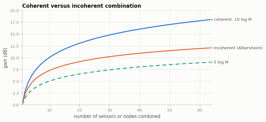
02 · Q1: do nodes hundreds of metres to kilometres apart beat a towed array?
Does an array of sonar transducers, separated by hundreds of metres or kilometres, provide sensitivity advantages for surface or underwater vessel detection, compared with conventional towed sonar arrays?
We separate the question into four parts, each with its own simulation:
- Array gain. Does spreading sensors out raise the gain against noise? (§1–2)
- Coherent combination across nodes. When, if ever, can widely spaced nodes add in phase? (§3)
- Detection coverage. Including the effect of sensors being closer to targets. (§4)
- Localisation. Where wide spacing clearly wins. (§5)
Every parameter cell is marked Parameters and can be edited and re-run.
Code
import sys, os
sys.path.insert(0, os.path.abspath('..'))
import numpy, scipy, matplotlib, PIL  # named here so the in-browser (JupyterLite) kernel loads them
import numpy as np
import matplotlib.pyplot as plt
from sonarsim import style, physics, arrays, imaging, modes, cases
style.use()
1. Array gain depends on the number of coherent elements, not the aperture
Two families of line arrays at 300 Hz (λ = 5 m), in spatially white noise:
- filled: λ/2 spacing, so the element count grows with length;
- sparse: always 16 elements, spread evenly over the same length.
With a perfectly coherent signal, the sparse array's gain stays at $10\log_{10}16 = 12$ dB however large it gets: spacing buys resolution, not gain. With a realistic coherence length the sparse array is worse still, because its elements fall outside each other's coherence.
Code
# Parameters
F_HZ = 300.0          # frequency
N_SPARSE = 16         # elements in the sparse array
LC_LAMBDA = 30        # signal coherence length in wavelengths (Carey number)

lam = 1500 / F_HZ
L = np.logspace(1, 4, 40)                 # aperture 10 m ... 10 km
filled_ideal, filled_lc, sparse_ideal, sparse_lc = [], [], [], []
for Li in L:
    g, n = arrays.array_gain_line_db(Li, F_HZ, np.inf); filled_ideal.append(g)
    filled_lc.append(arrays.array_gain_line_db(Li, F_HZ, LC_LAMBDA * lam)[0])
    pos = arrays.towed_line(Li, N_SPARSE, 100)
    sparse_ideal.append(arrays.array_gain_db(pos, F_HZ))
    sparse_lc.append(arrays.array_gain_db(pos, F_HZ, Lh=LC_LAMBDA * lam))

fig, ax = plt.subplots(figsize=(7.6, 4.0))
ax.semilogx(L, filled_ideal, color=style.BLUE, ls=(0, (4, 3)))
ax.semilogx(L, filled_lc, color=style.BLUE)
ax.semilogx(L, sparse_ideal, color=style.ORANGE, ls=(0, (4, 3)))
ax.semilogx(L, sparse_lc, color=style.ORANGE)
style.label_end(ax, L[-1], filled_ideal[-1], 'filled, perfectly coherent', style.BLUE)
style.label_end(ax, L[-1], filled_lc[-1], f'filled, Lc = {LC_LAMBDA} λ', style.BLUE)
style.label_end(ax, L[-1], sparse_ideal[-1], f'{N_SPARSE} elements, coherent', style.ORANGE)
style.label_end(ax, L[-1], sparse_lc[-1], f'{N_SPARSE} elements, Lc = {LC_LAMBDA} λ', style.ORANGE)
ax.axvline(LC_LAMBDA * lam, color=style.MUTED, lw=1)
ax.text(LC_LAMBDA * lam * 1.05, 1, f'Lc = {LC_LAMBDA*lam:.0f} m', fontsize=8.5, color=style.INK2)
ax.set_xlabel('aperture (m)'); ax.set_ylabel('array gain (dB)')
ax.set_ylim(0, 40); ax.set_xlim(10, 1e4)
ax.set_title(f'Array gain at {F_HZ:g} Hz: element count and coherence decide', loc='left')
style.save(fig, 'q1_gain_vs_aperture')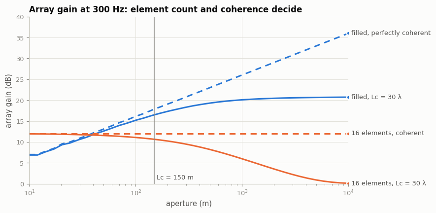
Reading the plot. A filled 1.5 km line at 300 Hz has about 600 elements and would give 28 dB if the ocean were perfectly coherent; with $L_c$ = 30 λ it gives about 20 dB. The sparse 16-element array starts at 12 dB and, summed coherently (delay-and-sum), falls towards 0 dB (one hydrophone's worth) once its spacing exceeds the coherence length, because a coherent sum of incoherent signals adds noise as fast as signal. Detecting at each element and fusing the outputs incoherently would keep about $5\log_{10}16 \approx 6$ dB instead; either way, spacing buys no gain.
2. How much gain does a real towed array keep?
Code
# Parameters
LENGTHS_M = [73, 300, 1500]           # TB-16 class, mid, SURTASS class
FREQS_HZ = [30, 100, 300, 1000]
LC_LIST = [20, 30, 100]               # coherence lengths in wavelengths

rows = []
for Lm in LENGTHS_M:
    for f in FREQS_HZ:
        ideal, n = arrays.array_gain_line_db(Lm, f, np.inf)
        vals = [arrays.array_gain_line_db(Lm, f, k * 1500 / f)[0] for k in LC_LIST]
        rows.append((Lm, f, n, ideal, *vals))
print(f"{'length':>7} {'freq':>6} {'elements':>9} {'ideal':>7} " + " ".join(f"{'Lc='+str(k)+'λ':>8}" for k in LC_LIST))
for r in rows:
    print(f"{r[0]:>6}m {r[1]:>5}Hz {r[2]:>9} {r[3]:>6.1f}  " + " ".join(f"{v:>8.1f}" for v in r[4:]))
length freq elements ideal Lc=20λ Lc=30λ Lc=100λ
73m 30Hz 3 4.8 4.7 4.7 4.8
73m 100Hz 10 10.0 9.6 9.8 9.9
73m 300Hz 30 14.8 13.8 14.1 14.6
73m 1000Hz 98 19.9 17.0 17.8 19.2
300m 30Hz 13 11.1 10.7 10.8 11.0
300m 100Hz 41 16.1 14.8 15.2 15.8
300m 300Hz 121 20.8 17.4 18.4 20.0
300m 1000Hz 401 26.0 18.6 20.1 23.6
1500m 30Hz 61 17.9 15.9 16.5 17.4
1500m 100Hz 201 23.0 18.1 19.3 21.7
1500m 300Hz 601 27.8 18.7 20.3 24.4
1500m 1000Hz 2001 33.0 18.9 20.7 25.6The long array is where coherence bites: the 1.5 km array gives up 3–9 dB of its ideal gain at 300 Hz and 7–14 dB at 1 kHz, depending on the coherence length. At 30 Hz the same array is only 15 wavelengths long and stays nearly coherent. This is the physical reason surveillance arrays are long and low-frequency.
3. Can kilometre-spaced nodes be combined coherently?
Take 9 nodes on a 3 × 3 grid, 5 km apart. If their signals were coherent, a coherent sum would focus with $10\log_{10}9 = 9.5$ dB of network gain. The fraction actually realised is $\frac{1}{M^2}\sum_{ij}\rho_{ij}$ with $\rho_{ij} = e^{-d_{ij}/L_c}$:
Code
# Parameters
N_NODES = 9
SPACING_M = 5000.0
freqs = np.logspace(0, 3, 60)          # 1 Hz ... 1 kHz

nodes = arrays.node_field(N_NODES, SPACING_M, 'grid')
fig, ax = plt.subplots(figsize=(7.6, 3.8))
for k, col in [(30, style.BLUE), (100, style.ORANGE)]:
    frac = [arrays.coherence_matrix(nodes, Lh=k * 1500 / f).sum() / N_NODES**2 for f in freqs]
    g = 10 * np.log10(np.array(frac) * N_NODES)   # coherent network gain actually obtained
    ax.semilogx(freqs, g, color=col, label=f'Lc = {k} λ')
ax.legend(loc='center right')
ax.axhline(10*np.log10(N_NODES), color=style.MUTED, lw=1, ls=(0, (4, 3)))
ax.text(1.1, 10*np.log10(N_NODES) + 0.3, f'perfect coherence: {10*np.log10(N_NODES):.1f} dB', fontsize=8.5, color=style.INK2)
ax.set_xlabel('frequency (Hz)'); ax.set_ylabel('coherent network gain (dB)')
ax.set_ylim(-0.5, 11); ax.set_xlim(1, 1000)
ax.set_title(f'{N_NODES} nodes {SPACING_M/1000:g} km apart: coherent gain across nodes', loc='left')
style.save(fig, 'q1_network_coherence')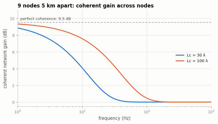
With $L_c$ = 30 λ the coherent network gain across 5 km-spaced nodes is under 1 dB above ~30 Hz; with an optimistic 100 λ it is still ~2.5 dB at 50 Hz and ~0.5 dB at 100 Hz. Incoherent fusion of the node outputs gives about $5\log_{10}M$ (4.8 dB for 9 equal nodes; see notebook 01) without any coherence, so a coherent sum is only worth attempting where it beats that: below ~8 Hz ($L_c$ = 30 λ) to ~28 Hz (100 λ). At those frequencies a 150 m shelf is close to modal cutoff, so the low-frequency end of this plot is a deep-water result.
Conclusion for sensitivity: widely spaced nodes add no array gain beyond what each node has on its own, plus a modest incoherent fusion gain. A towed array with hundreds of closely spaced hydrophones has 15–25 dB more gain than a single-hydrophone node.
4. Detection coverage: the proximity effect
Array gain is not the whole sonar equation. Distributed nodes are closer to wherever the target is, which cuts transmission loss. The model below compares, over a 20 km × 20 km box in 150 m-deep water:
- a 1.5 km towed array at the centre (30 m deep), with its coherence-limited gain in shallow-water ambient noise (wind and distant shipping, normal-mode model; see notebook 03, §2) and an optional self-noise penalty;
- 9 or 25 single-hydrophone nodes on a grid, fused incoherently.
Transmission loss is spherical to 150 m, cylindrical beyond, plus seawater absorption and 0.5 dB/km of bottom loss. Noise 65 dB re 1 µPa²/Hz (moderate shipping and sea state 3), bandwidth 100 Hz, 10 s integration, $P_d \approx 0.6$, $P_{fa}=10^{-4}$, steady (non-fading) signal. Source levels are swept, because modern submarine levels are not public and the comparison is more robust than any single number.
Code
# Parameters
F_HZ = 300.0
AREA_M = 20000.0
NL = 65.0                  # noise spectrum level, dB re 1 uPa^2/Hz
EXTRA_LOSS = 0.5           # bottom interaction loss, dB/km
TRANSITION_M = 150.0       # spherical -> cylindrical (water depth)
TOWED_SELF_NOISE_DB = 0.0  # extra noise on the towed array from its platform / flow (try 3-6 dB)
LC_LAMBDA = 30
SHIPPING_WEIGHT = 0.3      # ambient-noise mix: shipping power relative to wind (0 = wind only)
DT = physics.detection_threshold_db(bandwidth_hz=100, integration_s=10)

wg = modes.Pekeris(F_HZ, TRANSITION_M)
towed = arrays.towed_line(1500, arrays.half_wave_count(1500, F_HZ), 30)
AG_TOWED = arrays.array_gain_db(towed, F_HZ, Lh=LC_LAMBDA * 1500 / F_HZ,
                                noise=modes.modal_noise_csm(wg, towed, wind=1.0, shipping=SHIPPING_WEIGHT))
g = np.linspace(-AREA_M/2, AREA_M/2, 161)
X, Y = np.meshgrid(g, g)

def snr_map(sl, config):
    if config == 'towed':
        r = np.hypot(X, Y)
        return physics.passive_snr_db(sl, physics.transmission_loss(r, F_HZ, TRANSITION_M, EXTRA_LOSS),
                                      NL + TOWED_SELF_NOISE_DB, AG_TOWED)
    n = {'nodes9': 9, 'nodes25': 25}[config]
    nd = arrays.node_field(n, AREA_M / np.sqrt(n), 'grid')
    s = np.stack([physics.passive_snr_db(sl, physics.transmission_loss(np.hypot(X-x, Y-y), F_HZ, TRANSITION_M, EXTRA_LOSS), NL, 0.0)
                  for x, y, _ in nd])
    return physics.fuse_snr_db(s)

CONFIGS = [('towed', f'towed 1.5 km (AG {AG_TOWED:.1f} dB)', style.BLUE),
           ('nodes9', '9 single-hydrophone nodes', style.ORANGE),
           ('nodes25', '25 single-hydrophone nodes', style.RED)]
SL = np.arange(90, 136, 2.0)
cover = {c: [np.mean(snr_map(s, c) >= DT) for s in SL] for c, _, _ in CONFIGS}

fig, ax = plt.subplots(figsize=(7.6, 4.0))
for c, lab, col in CONFIGS:
    ax.plot(SL, 100 * np.array(cover[c]), color=col)
    i = int(np.argmin(np.abs(np.array(cover[c]) - 0.5)))
    style.label_end(ax, SL[i], 100 * cover[c][i], lab, col, dx=6)
ax.set_xlabel('target source level (dB re 1 µPa²/Hz at 1 m)'); ax.set_ylabel('area covered (%)')
ax.set_ylim(0, 102)
ax.set_title('Share of a 20 × 20 km box where the target is detected', loc='left')
style.save(fig, 'q1_coverage_vs_sl')
print(f"detection threshold DT = {DT:.1f} dB, towed array gain = {AG_TOWED:.1f} dB")
for c, lab, _ in CONFIGS:
    cv = np.array(cover[c]); print(f"  {lab:30s} 90% coverage from SL = {SL[np.argmax(cv >= 0.9)]:.0f} dB")
detection threshold DT = -9.0 dB, towed array gain = 22.1 dB towed 1.5 km (AG 22.1 dB) 90% coverage from SL = 102 dB 9 single-hydrophone nodes 90% coverage from SL = 116 dB 25 single-hydrophone nodes 90% coverage from SL = 112 dB
Code
# Parameters
SL_MAP = 106.0    # source level for the maps

fig, axs = plt.subplots(1, 3, figsize=(11.5, 3.9), sharey=True)
for ax, (c, lab, col) in zip(axs, CONFIGS):
    s = snr_map(SL_MAP, c) - DT
    im = ax.imshow(np.clip(s, -20, 20), extent=[-10, 10, -10, 10], origin='lower', cmap=style.DIV, vmin=-20, vmax=20)
    ax.contour(g/1000, g/1000, s, levels=[0], colors=[style.INK], linewidths=1)
    if c == 'towed':
        ax.plot([-0.75, 0.75], [0, 0], color=style.BLUE, lw=3)
    else:
        n = 9 if c == 'nodes9' else 25
        nd = arrays.node_field(n, AREA_M/np.sqrt(n), 'grid') / 1000
        ax.plot(nd[:, 0], nd[:, 1], 'o', color=col, ms=5, mec=style.SURFACE)
    ax.set_title(f'{lab}\n{100*np.mean(s>=0):.0f}% covered', loc='left', fontsize=9.5)
    ax.set_xlabel('km'); ax.grid(False)
axs[0].set_ylabel('km')
cb = fig.colorbar(im, ax=axs, shrink=0.85, pad=0.02); cb.set_label('signal excess (dB); black line = detection')
style.save(fig, 'q1_coverage_maps')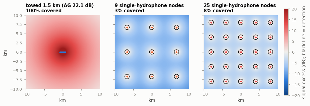
Reading the coverage results. The towed array covers 90% of the box against targets down to about 104 dB.
Nine single-hydrophone nodes need about 116 dB, a target 12 dB louder, and even 25 nodes need about 112 dB. Being
closer to the target does not make up for the missing array gain of single hydrophones at these ranges and
frequencies. That changes when each node is itself an array (notebook 04), when the towed array is noisy (try
TOWED_SELF_NOISE_DB = 6), or when transmission loss is steep (high frequency, lossy bottoms: try EXTRA_LOSS = 2).
5. Localisation: where wide spacing clearly wins
A towed array measures bearing. Its angular resolution is about λ/L; its range is unobserved in a single look unless the target is inside the near field ($\sim L^2/\lambda$), and a single line cannot tell left from right. Widely spaced nodes measure position, from arrival-time differences across long baselines.
The animations show both at 15 Hz (λ = 100 m), so the waves are visible at 16 km scale. A transient from the star spreads out; each sensor records it; the recordings are replayed time-reversed, and the re-emitted waves refocus on the source. The running maximum of that field is the delay-and-sum focused beamformer image.
Code
cases.show('plan_towed')The towed array focuses to a bearing band, not a point, with an identical mirror band on the other side of the line (left/right ambiguity). In the zoom, the band is about 400 m across, which is λ/L × range = 100 m / 1.5 km × 5.5 km, and it runs the full length of the bearing: range is unresolved.
Code
cases.show('plan_distributed')Nine coherent nodes 5 km apart focus to a spot about half a wavelength across (~50 m), with a sidelobe pattern of radial streaks around it: no ambiguity, and the position is fixed in one look. But this assumes the nodes are coherent, which §3 showed is realistic only below ~10–30 Hz. The next case adds random path errors of 40 m (0.4 λ) between nodes, a mild stand-in for the medium decorrelating the signal between sites:
Code
cases.show('plan_distributed_jitter')The coherent focus collapses (peak 0.44 instead of 1) and fragments. Without coherence, the nodes still localise by arrival-time differences (TDOA) of the signal envelope, which needs only that each node detect the same event. Accuracy is then set by timing precision, not wavelength. The map below is the Cramér–Rao bound for TDOA localisation with the 9-node grid, assuming each node times the arrival to 30 m-equivalent (20 ms): a pessimistic figure allowing for multipath.
Code
# Parameters
SIGMA_R_M = 30.0            # per-node timing error x c (m); the CRLB for 100 Hz bandwidth at 10 dB is ~2 m
nodes = arrays.node_field(9, 5000, 'grid')
gg = np.linspace(-12000, 12000, 241)
err = imaging.toa_fisher_rms(nodes, gg, gg, SIGMA_R_M)
fig, ax = plt.subplots(figsize=(5.6, 4.6))
from matplotlib.colors import LogNorm
im = ax.imshow(err, extent=[-12, 12, -12, 12], origin='lower', cmap=style.SEQ, norm=LogNorm(10, 1000))
cs = ax.contour(gg/1000, gg/1000, err, levels=[30, 50, 100, 300], colors=[style.INK2], linewidths=0.8)
ax.clabel(cs, fmt='%d m', fontsize=8)
ax.plot(nodes[:, 0]/1000, nodes[:, 1]/1000, 'o', color=style.ORANGE, ms=6, mec=style.SURFACE)
ax.set_xlabel('km'); ax.set_ylabel('km'); ax.grid(False)
cb = fig.colorbar(im, ax=ax, shrink=0.85); cb.set_label('RMS position error (m)')
ax.set_title('9 nodes, time-difference localisation', loc='left')
style.save(fig, 'q1_tdoa_error')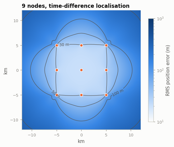
Inside the node field the position error is 20–40 m from a single event, degrading outside it. A single towed array gets bearing only; range needs either several minutes of own-ship manoeuvre (target motion analysis) or a second array.
Answer to Q1
For sensitivity, no. Array gain against noise comes from the number of sensors whose signals add coherently. The ocean keeps signals coherent over only ~20–40 wavelengths in shallow water (≈100–200 m at 300 Hz), so nodes hundreds of metres to kilometres apart cannot be added coherently across most of the passive band. Their outputs can only be fused incoherently, worth about $5\log_{10}M$ dB. Nine single-hydrophone nodes therefore have ~15 dB less combined gain than a 1.5 km towed array with ~600 hydrophones (20 dB coherence-limited), and in the coverage model they need a target ~12 dB louder to cover the same 20 × 20 km box, despite being closer to it.
For the system as a whole, it depends what is at each node. Spreading sensors out does bring real advantages: (i) proximity, which pays off when each node already has meaningful gain (notebook 04) or transmission loss is steep; (ii) localisation: position from one event, with no left/right ambiguity; (iii) freedom from tow-platform self-noise and the option to put sensors where propagation is best (below the layer, on the reliable acoustic path); (iv) for active sonar, multistatic geometry.
Coherent processing across nodes is physically possible only at very low frequency (≲10 Hz in shallow water, ≲30 Hz in deep water for 5 km spacing), where it would give a very sharp focus with ~1/M sidelobes, but still only $10\log_{10}(\text{total sensors})$ of gain.
03 · Q2: how do vertically suspended arrays compare with towed arrays?
What about vertically suspended sonar arrays — how do/would they compare to towed arrays?
A towed array is a horizontal line at one depth; a suspended array is a vertical line spanning part of the water column. The two see different things:
| Horizontal (towed) | Vertical (suspended) | |
|---|---|---|
| resolves | azimuth (bearing), with a left/right ambiguity | elevation (vertical arrival angle) |
| blind to | elevation (a cone of directions per beam) | azimuth: omnidirectional round the vertical axis |
| depth | one depth | many depths at once |
Five comparisons follow: array gain in the free-field (deep-water) picture of directional noise (§1) and in a shallow-water waveguide (§2), bearing (§3), coverage across a thermocline (§4), and telling a surface ship from a submarine (§5).
Code
import sys, os
sys.path.insert(0, os.path.abspath('..'))
import numpy, scipy, matplotlib, PIL  # named here so the in-browser (JupyterLite) kernel loads them
import numpy as np
import matplotlib.pyplot as plt
from sonarsim import style, physics, arrays, modes, cases
style.use()
1. Array gain in directional noise: the free-field (deep-water) picture
Both arrays have 32 elements at λ/2 (300 Hz, 77 m long). The noise field mixes wind noise from above (∝ sin elevation, with a fraction reflected from the bottom) with distant shipping near the horizontal (±6°, all azimuths). The target is a plane wave at broadside for the horizontal array and at the horizon for the vertical array. This is the classic deep-water picture, with a noise "notch" near the horizontal; §2 repeats the comparison in a shallow waveguide.
Code
# Parameters
F_HZ = 300.0
N_EL = 32
BOTTOM_REFLECTION = 0.3        # fraction of wind noise returned from the bottom (deep water ~0.1, shallow 0.3-0.5)
SHIP_WIDTH_DEG = 6.0           # half-width of the shipping-noise band around the horizon

lam = 1500 / F_HZ
hla = arrays.towed_line(lam/2*(N_EL-1), N_EL, 60)
vla = arrays.vertical_line(20, 20 + lam/2*(N_EL-1), N_EL)
ship = np.logspace(-2, 1, 25)          # shipping weight relative to wind
ag_h, ag_v = [], []
for s in ship:
    m = dict(wind=1.0, shipping=s, bottom_reflection=BOTTOM_REFLECTION, shipping_width_deg=SHIP_WIDTH_DEG)
    ag_h.append(arrays.array_gain_db(hla, F_HZ, noise='directional', noise_model=m, az_deg=90))
    ag_v.append(arrays.array_gain_db(vla, F_HZ, noise='directional', noise_model=m, az_deg=90))
# express the mix as the share of total noise power that is shipping
el = np.linspace(-89.5, 89.5, 359)
w = np.cos(np.deg2rad(el))
share = [np.sum(arrays.noise_directionality(el, wind=0, shipping=s, floor=0, shipping_width_deg=SHIP_WIDTH_DEG)*w) /
         np.sum(arrays.noise_directionality(el, wind=1, shipping=s, bottom_reflection=BOTTOM_REFLECTION, shipping_width_deg=SHIP_WIDTH_DEG)*w) for s in ship]
share = 100 * np.array(share)
fig, ax = plt.subplots(figsize=(7.6, 4.0))
ax.plot(share, ag_h, color=style.BLUE); style.label_end(ax, share[-1], ag_h[-1], 'horizontal (towed), broadside', style.BLUE)
ax.plot(share, ag_v, color=style.AQUA); style.label_end(ax, share[-1], ag_v[-1], 'vertical, steered horizontal', style.AQUA)
ax.axhline(10*np.log10(N_EL), color=style.MUTED, lw=1, ls=(0, (4, 3)))
ax.text(1, 10*np.log10(N_EL)+0.4, f'white noise: {10*np.log10(N_EL):.1f} dB', fontsize=8.5, color=style.INK2)
ax.set_xlabel('share of noise power from distant shipping (%)'); ax.set_ylabel('array gain (dB)')
ax.set_xlim(0, 100); ax.set_ylim(5, 27)
ax.set_title(f'{N_EL}-element arrays at {F_HZ:g} Hz in directional noise', loc='left')
style.save(fig, 'q2_gain_vs_noise_mix')
print(f"wind-only: horizontal {ag_h[0]:.1f} dB, vertical {ag_v[0]:.1f} dB;  shipping-dominated: horizontal {ag_h[-1]:.1f} dB, vertical {ag_v[-1]:.1f} dB")
wind-only: horizontal 14.1 dB, vertical 23.3 dB; shipping-dominated: horizontal 16.0 dB, vertical 7.5 dB
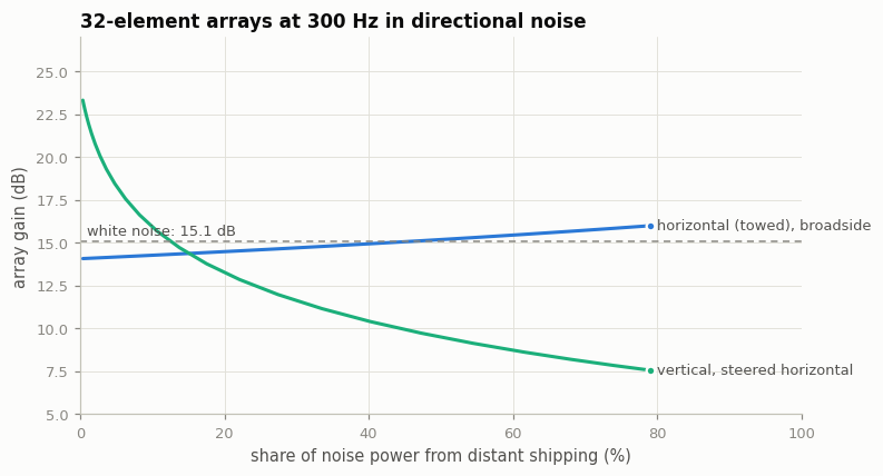
When wind noise dominates (quiet shipping, rough sea), the vertical array rejects the steep surface noise and gains ~9 dB more than the horizontal array. The horizontal array's broadside beam is a vertical fan that still takes noise from overhead. When distant shipping dominates, noise arrives near the horizontal from every azimuth, straight into the vertical array's horizontal beam, and the horizontal array wins by ~8 dB because it rejects shipping from other bearings. In this picture the answer depends on the noise environment: quiet, windy or remote deep waters favour the vertical array; busy shipping lanes favour the horizontal one. The vertical figures are upper bounds: they assume the whole signal arrives as one plane wave from the horizon, perfectly coherent down the array.
2. Array gain in a shallow-water waveguide
On a shelf both assumptions of §1 fail. The target's signal is a sum of normal modes, arriving at a spread of vertical angles up to the critical angle, so no single vertical beam collects all of it. And wind noise is carried to the array mainly by the same low-order modes (Kuperman & Ingenito 1980), which fills the deep-water notch. The model below uses the Pekeris waveguide of §5 (150 m of water over a sand-like bottom, 300 Hz, 28 modes) for both signal and noise:
- noise: Kuperman–Ingenito wind noise from a sheet of near-surface sources, plus distant shipping (sources beyond 10 km, which reach the array mostly in low-order modes), plus a white floor 20 dB down;
- horizontal array: 32 elements at λ/2, 30 m deep, plane-wave signal with the Carey coherence of notebook 02;
- vertical array: 32 elements spanning 10–140 m, signal = the modelled field of sources at 5–120 m depth and 2–10 km range, processed two ways: a fan of conventional plane-wave beams (best beam kept), or matched-field weights (the modelled field itself, which needs the environment and range to be known).
Code
# Parameters
WATER_DEPTH = 150.0
TOW_DEPTH = 30.0
LC_LAMBDA = 30

wg300 = modes.Pekeris(F_HZ, WATER_DEPTH)
hla_s = arrays.towed_line(lam/2*(N_EL-1), N_EL, TOW_DEPTH)
vla_s = arrays.vertical_line(10, WATER_DEPTH - 10, N_EL)
ship_s = np.logspace(-1.5, 1.5, 13)            # shipping power relative to wind
g_h, g_b, g_m = [], [], []
for s in ship_s:
    g_h.append(arrays.array_gain_db(hla_s, F_HZ, Lh=LC_LAMBDA*lam, noise=modes.modal_noise_csm(wg300, hla_s, 1.0, s)))
    gv = modes.vla_gain_db(wg300, vla_s[:, 2], modes.modal_noise_csm(wg300, vla_s, 1.0, s))
    g_b.append(gv['beam']); g_m.append(gv['matched'])
share_s = 100 * ship_s / (1 + ship_s)
fig, ax = plt.subplots(figsize=(7.6, 4.0))
ax.plot(share_s, g_h, color=style.BLUE); style.label_end(ax, share_s[-1], g_h[-1], 'horizontal (towed), broadside', style.BLUE)
ax.plot(share_s, g_m, color=style.AQUA); style.label_end(ax, share_s[-1], g_m[-1], 'vertical, matched-field', style.AQUA)
ax.plot(share_s, g_b, color=style.AQUA, ls=(0, (4, 3))); style.label_end(ax, share_s[-1], g_b[-1], 'vertical, plane-wave beams', style.AQUA)
ax.axhline(10*np.log10(N_EL), color=style.MUTED, lw=1, ls=(0, (4, 3)))
ax.text(1, 10*np.log10(N_EL)+0.4, f'white noise, plane wave: {10*np.log10(N_EL):.1f} dB', fontsize=8.5, color=style.INK2)
ax.set_xlabel('share of noise power from distant shipping (%)'); ax.set_ylabel('array gain (dB)')
ax.set_xlim(0, 100); ax.set_ylim(0, 20)
ax.set_title(f'{N_EL}-element arrays, {WATER_DEPTH:g} m shelf, {F_HZ:g} Hz (normal-mode model)', loc='left')
style.save(fig, 'q2_gain_shallow_water')
print(f"{wg300.nmodes} modes. Horizontal {min(g_h):.1f}-{max(g_h):.1f} dB; vertical matched-field {min(g_m):.1f}-{max(g_m):.1f} dB; "
      f"vertical plane-wave beams {min(g_b):.1f}-{max(g_b):.1f} dB")
28 modes. Horizontal 16.0-16.2 dB; vertical matched-field 13.1-14.2 dB; vertical plane-wave beams 6.8-12.0 dB
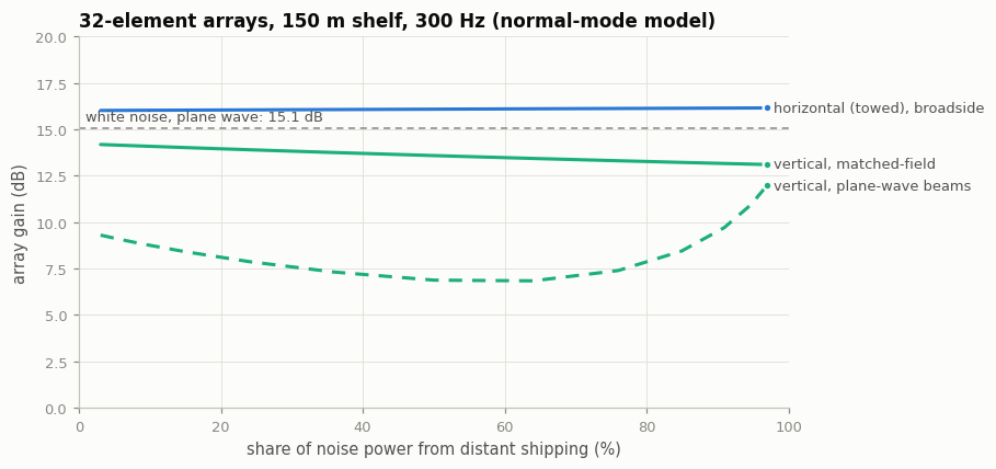
In shallow water the ranking flips. The horizontal array keeps ~16 dB whatever the noise mix. The vertical array loses its deep-water advantage: with plane-wave beams it keeps only ~7–12 dB (the high end only when shipping dominates), because the signal is spread over many modes and the noise shares those modes; matched-field processing recovers ~13–14 dB, still 2–3 dB below the horizontal array, and only if the environment is known well enough. Real vertical coherence is also imperfect (internal waves), which this model leaves out. So for sensitivity alone, a shelf favours the horizontal array.
3. Bearing: the vertical array has none
Code
az = np.linspace(0, 360, 721)
fig, axs = plt.subplots(1, 2, figsize=(10.5, 3.6), sharey=True)
for arr, col, lab in [(hla, style.BLUE, 'horizontal'), (vla, style.AQUA, 'vertical')]:
    w_ = arrays.steering(arr, F_HZ, 90, 0) / len(arr)
    bp = [np.abs(w_.conj() @ arrays.steering(arr, F_HZ, a, 0))**2 for a in az]
    axs[0].plot(az, 10*np.log10(np.maximum(bp, 1e-6)), color=col, label=lab)
    elv = np.linspace(-90, 90, 721)
    bp = [np.abs(w_.conj() @ arrays.steering(arr, F_HZ, 90, e))**2 for e in elv]
    axs[1].plot(elv, 10*np.log10(np.maximum(bp, 1e-6)), color=col, label=lab)
axs[0].set_xlabel('azimuth (deg), elevation 0'); axs[1].set_xlabel('elevation (deg), azimuth 90')
axs[0].set_ylabel('response (dB)'); axs[0].set_ylim(-40, 2)
axs[0].set_title('Response round the horizon', loc='left'); axs[1].set_title('Response in elevation', loc='left')
fig.legend(*axs[0].get_legend_handles_labels(), loc='upper center', ncol=2, bbox_to_anchor=(0.5, 1.06)); axs[0].set_xlim(0, 360); axs[1].set_xlim(-90, 90)
axs[0].annotate('mirror beam\n(left/right ambiguity)', (270, 0), (190, -14), fontsize=8.5, color=style.INK2,
                arrowprops=dict(arrowstyle='-', color=style.MUTED))
style.save(fig, 'q2_beam_patterns')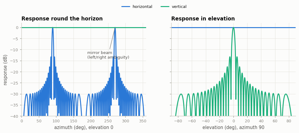
The horizontal array steered to 90° has an equal beam at 270°, its left/right ambiguity. The vertical array responds equally to every azimuth, so a single vertical array gives no bearing. It resolves elevation instead, which a horizontal array at broadside cannot. Bearing from vertical arrays therefore needs several of them (notebook 04), a horizontal arm, or directional (vector) sensors.
4. Coverage across a thermocline
The FDTD runs below simulate a 150 m-deep shelf at 100 Hz: a 40 m mixed layer at 18 °C over a thermocline to 10 °C at 80 m, a sandy sediment, and a sea surface. A 48-element vertical array spans 5–145 m at 3.5 km range; a single hydrophone at 30 m stands in for a towed array at a typical tow depth. The right-hand panel of each movie builds up the energy received at each depth.
Code
cases.show('section_surface_ship')Code
cases.show('section_sub_below_layer')Code
# Energy received at each depth for the two sources (from the saved FDTD traces)
fig, ax = plt.subplots(figsize=(5.2, 4.6))
res = {}
for name, col, lab in [('section_surface_ship', style.ORANGE, 'surface ship, 5 m'),
                       ('section_sub_below_layer', style.VIOLET, 'submarine, 90 m')]:
    d = np.load(f'../renders/{name}_traces.npz')
    n = int(d['vla_elements']); E = (d['traces']**2).sum(1); z = d['depths']
    mean = E[:n].mean()                       # water-column average (what a range-only TL model assumes)
    Edb = 10*np.log10(E[:n] / mean)
    ax.plot(Edb, z[:n], color=col, label=lab)
    tow = 10*np.log10(E[n] / mean)
    ax.plot([tow], [z[n]], 'o', color=col, mec=style.SURFACE, ms=7)
    res[lab] = (tow, 10*np.log10(E[:n].max() / mean))
ax.axvline(0, color=style.MUTED, lw=1)
ax.axhline(30, color=style.BLUE, lw=1, ls=(0, (2, 2))); ax.text(-9.6, 28, 'tow depth 30 m', fontsize=8.5, color=style.INK2)
ax.axhspan(40, 80, color=style.GRID, alpha=0.6, lw=0); ax.text(-9.6, 62, 'thermocline', fontsize=8.5, color=style.INK2)
ax.set_ylim(150, 0); ax.set_xlim(-10, 8)
ax.set_xlabel('received energy (dB re water-column average)'); ax.set_ylabel('depth (m)')
ax.legend(loc='lower left'); ax.set_title('Where the energy arrives', loc='left')
style.save(fig, 'q2_energy_by_depth')
for k, (tow, best) in res.items():
    print(f"{k:18s}: hydrophone at 30 m {tow:+5.1f} dB, best depth {best:+5.1f} dB, relative to the water-column average")
surface ship, 5 m : hydrophone at 30 m +0.9 dB, best depth +2.5 dB, relative to the water-column average submarine, 90 m : hydrophone at 30 m -1.9 dB, best depth +5.2 dB, relative to the water-column average
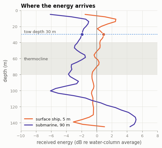
For the submarine below the layer the energy concentrates in the lower water column: a sensor at 30 m sits about 7 dB below the best depth, but only ~2 dB below the water-column average; for the surface ship it is ~1 dB above average. A vertical array's output follows the average energy over its aperture, so a full-column array is insensitive to where the layer is, while a fixed-depth array gains or loses a few dB depending on which side of the layer the target is. The effect is real but modest at this range; a towed array can also be lowered below the layer (at the cost of targets above it). (2D runs: levels are for line sources, but the depth distribution is the physically meaningful part.)
5. Surface ship or submarine? Depth discrimination
In a waveguide the depth structure of the received field encodes the source depth. A vertical array samples it directly; matched-field processing compares the data with modelled fields for each trial depth. The model is a Pekeris waveguide (100 m water over a fast sediment, 200 Hz, 13 propagating modes), source at 5 km, 0 dB SNR per element, 20 snapshots, range assumed known.
Code
# Parameters
F_HZ = 200.0
WATER_DEPTH = 100.0
RANGE_M = 5000.0
SNR_DB = 0.0
SOURCES = [5.0, 50.0]                   # surface ship, submarine

wg = modes.Pekeris(F_HZ, WATER_DEPTH)
zg = np.arange(1, WATER_DEPTH, 1.0)
lam = 1500 / F_HZ
geoms = {
    'vertical, 24 elements 5-95 m':  (np.linspace(5, 95, 24), np.full(24, RANGE_M), style.AQUA),
    'horizontal at 50 m, broadside': (np.full(64, 50.0), np.full(64, RANGE_M), style.BLUE),
    'horizontal at 50 m, endfire':   (np.full(64, 50.0), RANGE_M + np.arange(64) * lam / 2, style.VIOLET),
}
fig, axs = plt.subplots(1, 2, figsize=(10.5, 4.0), sharey=True)
for ax, zs in zip(axs, SOURCES):
    for lab, (rz, rr, col) in geoms.items():
        b = modes.mfp_depth(wg, zs, rz, rr, zg, snr_db=SNR_DB)
        ax.plot(10*np.log10(b / b.max()), zg, color=col, label=lab)
    ax.axhline(zs, color=style.INK, lw=1, ls=(0, (2, 2)))
    ax.set_title(f'true source depth {zs:g} m', loc='left')
    ax.set_xlabel('matched-field output (dB)'); ax.set_xlim(-15, 0.5)
axs[0].set_ylim(WATER_DEPTH, 0); axs[0].set_ylabel('trial source depth (m)')
axs[1].legend(loc='lower left', fontsize=8)
style.save(fig, 'q2_depth_discrimination')
print(f"{wg.nmodes} propagating modes")
13 propagating modes
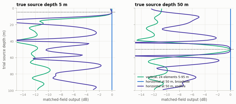
The vertical array's output peaks sharply at the true depth for both sources: it tells the 5 m surface ship from the 50 m submarine directly. The broadside horizontal array's output is flat: every element sees the same field, so it carries no depth information. At endfire the horizontal array can also resolve depth, through the different horizontal wavenumbers of the modes, but only for targets near its axis, which is also where towed arrays suffer most from tow-platform noise. Real environments are less well known than this model, which widens the peaks, but the contrast between the geometries holds (published VLA results: see notebook 01, §5).
Practical comparison
| Towed (horizontal) | Suspended (vertical) | |
|---|---|---|
| Gain, deep water | ~10 log N; best in shipping noise | up to ~10 log N + notch rejection when wind noise dominates |
| Gain, shallow water | ~10 log N, limited by horizontal coherence | 2–3 dB less (matched-field) to 4–9 dB less (plane-wave beams) |
| Bearing | yes, with left/right ambiguity (twin lines resolve it) | none from one array |
| Range | only near field or by own-ship manoeuvre | matched-field range and depth from one array (needs a good environment model) |
| Depth / classification | only near endfire | yes: surface vs submerged |
| Thermocline | one depth; ±1–2 dB here depending on the side of the layer | spans it; insensitive to layer depth |
| Self-noise | tow platform and flow noise, worst forward | none from towing; strumming and suspension motion instead |
| Aperture | up to ~1.5 km; limited by handling and coherence | limited by water depth and suspension |
| Mobility | moves with the ship | fixed or drifting; many needed for area coverage |
Answer to Q2
A vertical array trades bearing for depth. For equal element counts its gain depends on the water:
- in deep water, where noise has a notch near the horizontal, it can beat a horizontal array by up to ~9 dB when wind noise dominates, and loses by ~8 dB where distant shipping dominates (§1, upper bounds);
- on a shelf, it has 2–3 dB less gain than a horizontal array with matched-field processing and a well-known environment, and 4–9 dB less with conventional beams (§2).
Its real advantages are information, not gain: it spans the water column, so it is insensitive to the layer (a fixed-depth array gains or loses 1–2 dB here); it can tell surface ships from submarines and estimate range from a single array, which towed arrays mostly cannot; and it has no tow noise. It gives no bearing on its own and does not move, so it complements towed arrays rather than replacing them. The combination points to Q3: several vertical arrays, whose shared geometry supplies the bearing.
04 · Q3: what if each distributed node is a vertical array?
What if each of the sonar nodes in Q1 are vertical arrays, does that offer desirable traits?
Notebooks 02 and 03 found complementary strengths and gaps:
- widely spaced single hydrophones localise well but lack array gain, so they cover little area against quiet targets;
- a vertical array has gain, spans the layer and measures source depth, but gives no bearing.
A network of vertical arrays (VLA nodes) should combine the two: each node brings its own array gain and depth information, and the network geometry supplies the horizontal position. This notebook tests that with three simulations: coverage (§1), coverage when the target hides below the layer (§2), and surface/submerged classification from a VLA node whose range comes from the network (§3).
Code
import sys, os
sys.path.insert(0, os.path.abspath('..'))
import numpy, scipy, matplotlib, PIL  # named here so the in-browser (JupyterLite) kernel loads them
import numpy as np
import matplotlib.pyplot as plt
from sonarsim import style, physics, arrays, modes, imaging
style.use()
1. Detection coverage with array gain at every node
The same 20 × 20 km box, 150 m shelf, noise level, bandwidth and propagation as notebook 02. Each VLA node has 32 elements spanning 10–140 m. Its gain comes from the shallow-water normal-mode model of notebook 03 (§2), for the chosen noise mix, with two kinds of processing: conventional plane-wave beams, and matched-field processing (needs a known environment). The towed array's gain is computed in the same noise field.
The depth structure from the FDTD runs (notebook 03, §4) is applied on top of the range-only transmission loss: each configuration receives the average energy over its depth span, relative to the water-column average, for a surface ship (5 m) and for a submarine below the layer (90 m).
Code
# Parameters
F_HZ = 300.0
AREA_M = 20000.0
WATER_DEPTH = 150.0
NL = 65.0
EXTRA_LOSS = 0.5
SHIPPING_WEIGHT = 0.3       # noise mix: shipping power relative to wind (0 = wind only; 3 = shipping-dominated)
N_VLA_EL = 32
N_NODES = 9
LC_LAMBDA = 30
TOW_DEPTH = 30.0            # also the depth of the single-hydrophone nodes
TOWED_SELF_NOISE_DB = 0.0
DT = physics.detection_threshold_db(100, 10)

lam = 1500 / F_HZ
wg = modes.Pekeris(F_HZ, WATER_DEPTH)
vla = arrays.vertical_line(10, WATER_DEPTH - 10, N_VLA_EL)
R_VLA = modes.modal_noise_csm(wg, vla, 1.0, SHIPPING_WEIGHT)
# (FDTD case, source depth) for each scenario; the VLA gain depends on source depth, so compute it per scenario
SCENARIOS = {'surface ship, 5 m': ('section_surface_ship', 5.0),
             'submarine below the layer, 90 m': ('section_sub_below_layer', 90.0)}
G_VLA = {scen: modes.vla_gain_db(wg, vla[:, 2], R_VLA, source_depths=(zs,)) for scen, (_, zs) in SCENARIOS.items()}
towed = arrays.towed_line(1500, arrays.half_wave_count(1500, F_HZ), TOW_DEPTH)
AG_TOWED = arrays.array_gain_db(towed, F_HZ, Lh=LC_LAMBDA * lam,
                                noise=modes.modal_noise_csm(wg, towed, 1.0, SHIPPING_WEIGHT))
print(f"towed array gain {AG_TOWED:.1f} dB ({len(towed)} hydrophones)")
for scen, gv in G_VLA.items():
    print(f"VLA node gain, {scen}: {gv['beam']:.1f} dB plane-wave beams, {gv['matched']:.1f} dB matched-field ({N_VLA_EL} hydrophones)")

def depth_factor_db(case, z_lo, z_hi):
    # mean FDTD energy over [z_lo, z_hi] relative to the water-column mean
    d = np.load(f'../renders/{case}_traces.npz')
    n = int(d['vla_elements']); E = (d['traces']**2).sum(1); z = d['depths']   # VLA elements, then the 30 m hydrophone
    if z_hi - z_lo < 1:                                     # a single depth: nearest receiver
        e = E[np.argmin(np.abs(z - z_lo))]
    else:
        e = E[:n][(z[:n] >= z_lo - 1) & (z[:n] <= z_hi + 1)].mean()
    return 10*np.log10(e / E[:n].mean())

g = np.linspace(-AREA_M/2, AREA_M/2, 161)
X, Y = np.meshgrid(g, g)

def snr_map(sl, ag, n_nodes=None, self_noise=0.0, depth_db=0.0):
    if n_nodes is None:
        r = np.hypot(X, Y)
        return physics.passive_snr_db(sl, physics.transmission_loss(r, F_HZ, WATER_DEPTH, EXTRA_LOSS), NL + self_noise, ag) + depth_db
    nd = arrays.node_field(n_nodes, AREA_M/np.sqrt(n_nodes), 'grid')
    s = np.stack([physics.passive_snr_db(sl, physics.transmission_loss(np.hypot(X-x, Y-y), F_HZ, WATER_DEPTH, EXTRA_LOSS), NL, ag)
                  for x, y, _ in nd]) + depth_db
    return physics.fuse_snr_db(s)

# (label, kwargs, depth span, colour, line style)
CONFIGS = [
    ('towed 1.5 km', dict(ag=AG_TOWED, self_noise=TOWED_SELF_NOISE_DB), (TOW_DEPTH, TOW_DEPTH), style.BLUE, '-'),
    (f'{N_NODES} single-hydrophone nodes', dict(ag=0.0, n_nodes=N_NODES), (TOW_DEPTH, TOW_DEPTH), style.ORANGE, '-'),
    (f'{N_NODES} VLA nodes, matched-field', dict(ag='matched', n_nodes=N_NODES), (10, WATER_DEPTH - 10), style.YELLOW, '-'),
    (f'{N_NODES} VLA nodes, plane-wave beams', dict(ag='beam', n_nodes=N_NODES), (10, WATER_DEPTH - 10), style.YELLOW, (0, (4, 3))),
]
SL = np.arange(90, 132, 1.0)
towed array gain 22.1 dB (601 hydrophones) VLA node gain, surface ship, 5 m: 5.6 dB plane-wave beams, 13.6 dB matched-field (32 hydrophones) VLA node gain, submarine below the layer, 90 m: 8.8 dB plane-wave beams, 14.0 dB matched-field (32 hydrophones)
Code
fig, axs = plt.subplots(1, 2, figsize=(11.5, 4.0), sharey=True)
summary = {}
for ax, (scen, (case, _)) in zip(axs, SCENARIOS.items()):
    for lab, kw, span, col, ls in CONFIGS:
        dd = depth_factor_db(case, *span)
        if isinstance(kw['ag'], str):                       # VLA gain for this scenario's source depth
            kw = dict(kw, ag=G_VLA[scen][kw['ag']])
        cov = np.array([np.mean(snr_map(s, depth_db=dd, **kw) >= DT) for s in SL])
        ax.plot(SL, 100*cov, color=col, ls=ls, label=lab)
        summary[(scen, lab)] = (SL[np.argmax(cov >= 0.9)] if (cov >= 0.9).any() else np.nan, dd)
    ax.set_xlabel('target source level (dB re 1 µPa²/Hz at 1 m)')
    ax.set_title(scen, loc='left')
    ax.set_ylim(0, 102)
axs[0].set_ylabel('area covered (%)'); axs[0].legend(loc='lower right', fontsize=8.5)
style.save(fig, 'q3_coverage_vs_sl')
print('Quietest source level covered over 90% of the box (depth factor applied):')
for scen in SCENARIOS:
    print(f'  {scen}')
    for lab, *_ in CONFIGS:
        sl, dd = summary[(scen, lab)]
        print(f'    {lab:38s} {sl:5.0f} dB   (depth factor {dd:+.1f} dB)')
Quietest source level covered over 90% of the box (depth factor applied):
surface ship, 5 m
towed 1.5 km 101 dB (depth factor +0.9 dB)
9 single-hydrophone nodes 114 dB (depth factor +0.9 dB)
9 VLA nodes, matched-field 101 dB (depth factor +0.0 dB)
9 VLA nodes, plane-wave beams 109 dB (depth factor +0.0 dB)
submarine below the layer, 90 m
towed 1.5 km 104 dB (depth factor -1.9 dB)
9 single-hydrophone nodes 117 dB (depth factor -1.9 dB)
9 VLA nodes, matched-field 101 dB (depth factor -0.3 dB)
9 VLA nodes, plane-wave beams 106 dB (depth factor -0.3 dB)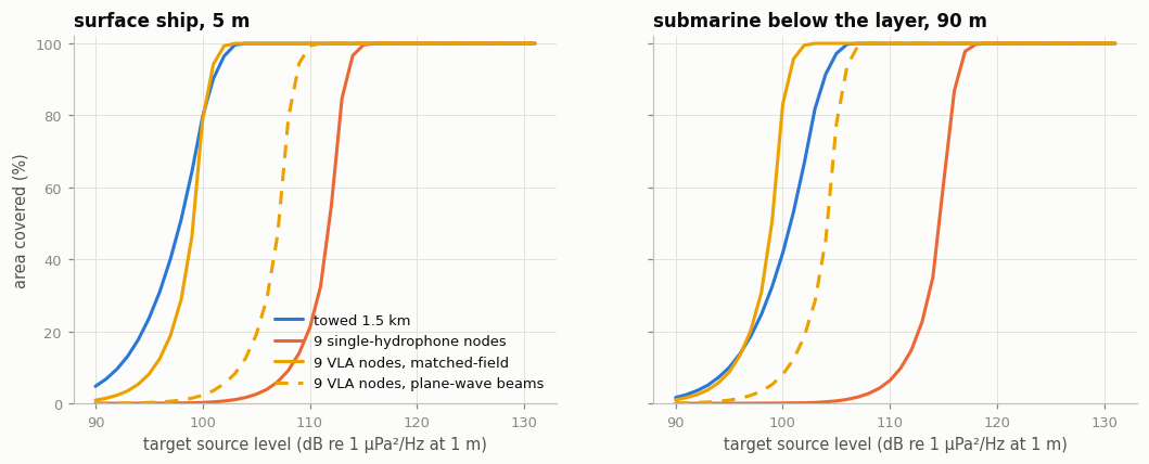
With matched-field processing, 9 VLA nodes reach parity with the 1.5 km towed array for the surface ship (both ~101 dB) and are ~3 dB ahead for the submarine below the layer, where the fixed-depth towed array sits in the weaker part of the column. These matched-field figures are an upper bound: they assume the environment and range are known and the modal field is perfectly coherent down the array, while the towed array carries the coherence loss measured at sea. With conventional plane-wave beams the VLA nodes need a target ~2–8 dB louder than the towed array (worst for the surface ship, whose energy sits in high-angle modes). Either way they are far ahead of single-hydrophone nodes (~8–16 dB).
Notes on fairness: 9 VLA nodes use 288 hydrophones against the towed array's 601; the towed array here has no self
noise (try TOWED_SELF_NOISE_DB = 3 to 6, typical of real tows, which moves the balance towards the VLA network);
the towed array moves and can sweep a larger area over time; and the result depends on the noise mix (try
SHIPPING_WEIGHT = 3).
2. Three-dimensional localisation
The network measures horizontal position by arrival-time differences (notebook 02, §5); each VLA measures depth, and from the depth structure also range. Together they give a 3D fix from a single event. The fix is also consistent across nodes, which is a strong check against false alarms.
3. Classification: surface or submerged?
A practical benefit of depth: most contacts in busy waters are surface ships. A node that can say "this source is at 5 m" can drop it before it reaches an operator. The Monte Carlo below places sources at random: half surface ships (2–8 m depth), half submarines (30–90 m), at 2–8 km from a VLA node in a Pekeris waveguide at 200 Hz. The network supplies the range with a ±150 m error; the VLA estimates depth by matched-field processing over depth and a ±300 m range window, and the contact is called submerged if the estimate is deeper than 20 m.
Code
# Parameters
F_HZ = 200.0
WATER_DEPTH = 100.0
N_EL = 24
TRIALS = 120                 # per SNR point (raise for smoother curves)
SNRS = [-15, -10, -5, 0, 5]  # per-element SNR, dB
RANGE_ERR_M = 150.0
SPLIT_M = 20.0

wg = modes.Pekeris(F_HZ, WATER_DEPTH)
rz = np.linspace(5, 95, N_EL)
zg = np.arange(1, WATER_DEPTH, 2.0)
rng = np.random.default_rng(7)

def classify(zs, r, snr):
    d = wg.field(zs, rz, [r])[:, 0]
    sig = np.linalg.norm(d)**2 / N_EL
    nv = sig / 10**(snr/10)
    R = np.zeros((N_EL, N_EL), complex)
    for _ in range(10):
        a = (rng.standard_normal() + 1j*rng.standard_normal()) / np.sqrt(2)
        x = a*d + np.sqrt(nv/2)*(rng.standard_normal(N_EL) + 1j*rng.standard_normal(N_EL))
        R += np.outer(x, x.conj())
    r_est = r + rng.normal(0, RANGE_ERR_M)
    rr = r_est + np.arange(-300, 301, 25.0)
    best, bz = -1, None
    for z in zg:
        rep = wg.field(z, rz, rr)                       # (N_EL, ranges)
        rep = rep / np.linalg.norm(rep, axis=0)
        b = np.real(np.einsum('nr,nm,mr->r', rep.conj(), R, rep)).max()
        if b > best:
            best, bz = b, z
    return bz

acc = []
for snr in SNRS:
    ok = 0
    for t in range(TRIALS):
        sub = t % 2 == 1
        zs = rng.uniform(30, 90) if sub else rng.uniform(2, 8)
        r = rng.uniform(2000, 8000)
        ok += ((classify(zs, r, snr) > SPLIT_M) == sub)
    acc.append(100 * ok / TRIALS)
fig, ax = plt.subplots(figsize=(6.6, 3.8))
ax.plot(SNRS, acc, 'o-', color=style.AQUA, ms=7, mec=style.SURFACE)
for s, a in zip(SNRS, acc):
    ax.annotate(f'{a:.0f}%', (s, a), xytext=(0, 8), textcoords='offset points', ha='center', fontsize=8.5, color=style.INK2)
ax.axhline(50, color=style.MUTED, lw=1, ls=(0, (4, 3))); ax.text(SNRS[0], 52, 'chance', fontsize=8.5, color=style.INK2)
ax.set_xlabel('SNR per hydrophone (dB)'); ax.set_ylabel('correct surface/submerged calls (%)')
ax.set_ylim(40, 105)
ax.set_title(f'VLA node, {N_EL} elements: surface vs submerged', loc='left')
style.save(fig, 'q3_classification')
print(dict(zip(SNRS, np.round(acc, 1))))
{-15: np.float64(65.8), -10: np.float64(92.5), -5: np.float64(99.2), 0: np.float64(100.0), 5: np.float64(98.3)}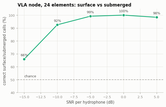
At −10 dB per hydrophone (about +4 dB after 24-element processing) the node calls 92% of contacts correctly, and from −5 dB it is essentially perfect in this idealised waveguide; at −15 dB it falls to 66%, heading for chance. In real water, uncertainty in the sound-speed profile and bottom degrades matched-field processing; robust variants (mode filtering, depth discrimination by interference striations) are the published response (notebook 01, §5).
4. Coherent processing across VLA nodes
Nothing about vertical arrays changes the horizontal coherence limit from Q1: nodes kilometres apart combine coherently only below ~8–30 Hz. VLA nodes do help a very-low-frequency coherent network in one way: each node can steer to a chosen vertical arrival angle before the nodes are combined, rejecting surface noise and multipath that would otherwise decorrelate the inter-node signal.
Answer to Q3
Yes, a network of vertical arrays has most of the desirable traits of both parent designs:
- Sensitivity comparable to a long towed array: on a shelf each node brings ~6–14 dB of array gain (plane-wave beams to matched-field), and the network adds proximity and incoherent fusion. In the model, 9 VLA nodes with matched-field processing cover a 20 × 20 km box as well as a 1.5 km towed array, ~3 dB better when the target is below the layer (an upper bound: known environment and range, no vertical-coherence loss); with conventional beams they are ~2–8 dB worse (§1). In deep water with a noise notch near the horizontal the VLA gain, and so the balance, can be higher (notebook 03, §1).
- Insensitive to the layer: every node spans the water column, so the answer does not depend on which side of the thermocline the target is (§1, right).
- 3D localisation from one event: horizontal position from the network, depth (and range) from each VLA.
- Classification: surface or submerged from each node's depth estimate, which cuts false alarms (§3).
- No left/right ambiguity, no tow noise, quiet deep deployment possible (TRAPS-style, notebook 01).
What it does not give is coherent array gain between nodes at normal passive frequencies; that limit is set by the ocean, not the hardware. The sensitivity gain over a towed array is also modest: roughly parity, with the edge depending on processing, noise and tow self-noise. The case for the concept rests on what it adds at equal sensitivity: 3D position, classification and layer robustness. The costs are practical: many moorings or drifting buoys, power and communications per node, suspension motion and strumming, and a fixed geometry that cannot chase a contact.
06 · What drives sonar performance: design parameters
The earlier notebooks compared specific configurations. This one pulls out the parameters that decide which configuration wins, and uses them to sketch what a good system looks like:
- Coherence sets a ceiling on array gain (§1).
- Frequency trades gain and resolution against absorption, bottom loss and target signature; for a given aperture and range there is a best frequency (§2).
- The thermocline matters a lot in some regimes and little in others; a parabolic-equation (PE) model maps it in deep water and on a shelf at 100 Hz, 1 kHz and 3.5 kHz (§3).
- Rigid (hull) arrays and an ideal-design sketch (§4).
Code
import sys, os
sys.path.insert(0, os.path.abspath('..'))
import numpy, scipy, matplotlib, PIL  # named here so the in-browser (JupyterLite) kernel loads them
import numpy as np
import matplotlib.pyplot as plt
from sonarsim import style, physics, arrays, cases, pe
style.use()
1. Coherence: the ceiling on array gain
The ocean keeps a signal in step over a coherence length $L_c$, which scales with wavelength: about 20–40 λ on continental shelves (Carey), longer on clean deep-water paths. With exponential decorrelation, the gain of a λ/2-sampled line grows as $10\log_{10}N$ while it is shorter than $L_c$ and then flattens towards $10\log_{10}(4L_c/\lambda)$, whatever its length.
Code
# Parameters
LC_LIST = [20, 30, 100]          # coherence lengths in wavelengths
F_HZ = 300.0

lam = 1500 / F_HZ
L_lam = np.logspace(0, np.log10(3000), 60)     # aperture in wavelengths
fig, ax = plt.subplots(figsize=(7.6, 4.0))
ax.semilogx(L_lam, [arrays.array_gain_line_db(x * lam, F_HZ, np.inf)[0] for x in L_lam], color=style.MUTED, ls=(0, (4, 3)))
style.label_end(ax, L_lam[-1], arrays.array_gain_line_db(L_lam[-1] * lam, F_HZ, np.inf)[0], 'perfectly coherent', style.MUTED)
for k, col in zip(LC_LIST, [style.ORANGE, style.BLUE, style.AQUA]):
    g = [arrays.array_gain_line_db(x * lam, F_HZ, k * lam)[0] for x in L_lam]
    ax.semilogx(L_lam, g, color=col)
    style.label_end(ax, L_lam[-1], g[-1], f'Lc = {k} λ (ceiling {10*np.log10(4*k):.0f} dB)', col)
    ax.axvline(k, color=col, lw=0.8, ls=(0, (2, 3)))
ax.set_xlabel('array length (wavelengths)'); ax.set_ylabel('array gain, white noise (dB)')
ax.set_ylim(0, 40); ax.set_xlim(1, 3000)
ax.set_title('Gain saturates once the array is longer than the coherence length', loc='left')
style.save(fig, 'd_coherence_ceiling')
for k in LC_LIST:
    print(f"Lc = {k:3d} lambda: ceiling {10*np.log10(4*k):.1f} dB; a {k}-lambda array reaches "
          f"{arrays.array_gain_line_db(k * lam, F_HZ, k * lam)[0]:.1f} dB, a {10*k}-lambda array "
          f"{arrays.array_gain_line_db(10 * k * lam, F_HZ, k * lam)[0]:.1f} dB")
Lc = 20 lambda: ceiling 19.0 dB; a 20-lambda array reaches 14.8 dB, a 200-lambda array 18.6 dB Lc = 30 lambda: ceiling 20.8 dB; a 30-lambda array reaches 16.5 dB, a 300-lambda array 20.3 dB Lc = 100 lambda: ceiling 26.0 dB; a 100-lambda array reaches 21.7 dB, a 1000-lambda array 25.6 dB
What sets $L_c$:
- the medium: internal waves and sound-speed fluctuations scramble phase, more so at longer range, higher frequency and on summer shelves with a sharp thermocline;
- boundaries: rough sea surface and seabed scatter the signal; bottom-interacting paths decorrelate fastest;
- multipath and modes: interference between paths varies from point to point. In the vertical this structure is deterministic and recoverable with matched-field processing (notebook 03); horizontal decorrelation is random;
- the platform: unknown element positions (towed-array shape) act like a loss of coherence; errors must be below about λ/10 (notebook 07, §4);
- time: target manoeuvres, Doppler and medium changes limit how long a narrowband signal can be integrated.
A longer array beyond one or two coherence lengths buys resolution (narrower beams, range focusing), not sensitivity. More sensitivity needs more coherent hydrophones inside a coherence length: more elements per wavelength² (planar or volumetric arrays) or lower frequency (longer $L_c$ in metres).
2. Choosing the frequency
For a fixed aperture the frequency trades several effects against each other:
| Low (10–500 Hz) | Mid (0.5–5 kHz) | High (5–100 kHz) | |
|---|---|---|---|
| Absorption | ~0.001–0.02 dB/km | 0.02–0.3 dB/km | 0.3–30 dB/km |
| Target signal | strongest; machinery and blade-rate tonals | broadband flow and propeller noise; quiet on modern submarines | weak passively; active imaging |
| Dominant noise | distant shipping | wind (falls ~5–6 dB/octave) | wind, then thermal |
| Element spacing λ/2 | 1.5–75 m | 0.15–1.5 m | 7.5 mm–15 cm |
| Aperture for a ~2° beam (~30 λ) | 90 m–4.5 km | 9–90 m | 0.5–9 m |
| Layer and seabed | leaks through the layer; bottom reflects well | trapped in the layer; more bottom loss | stays near the surface |
| Active projectors | large and heavy (~λ/2 across) | ship-sized | compact |
An illustrative figure of merit captures the core trade for a passive array of fixed size:
$$\mathrm{FOM}(f) = AG(f) + s\,\log_2(f/1\,\text{kHz}) - \alpha(f)R - b\,(f/1\,\text{kHz})\,R$$
$AG$ grows ~3 dB/octave for a line (6 dB for a square planar array) until the array is a coherence length long; $s$ is how fast the target spectrum falls relative to the noise (target falls ~6 dB/octave, wind noise ~5, so ~−1); $\alpha$ is seawater absorption; $b$ is a frequency-proportional bottom loss for shelf water. The best frequency is where the FOM peaks.
Code
# Parameters
S_DB_PER_OCTAVE = -1.0            # target spectrum slope minus noise slope
CAREY = 30                        # coherence length, wavelengths
SHELF_BOTTOM_DB_PER_KM_PER_KHZ = 0.3
APERTURES = [                     # (label, kind, size m)
    ('2 m square (small USV hull)', 'planar', 2.0),
    ('5 m square (ship bow array)', 'planar', 5.0),
    ('40 m line (submarine flank)', 'line', 40.0),
    ('300 m line (short towed)', 'line', 300.0),
    ('1.5 km line (long towed)', 'line', 1500.0),
]
RANGES_KM = np.logspace(0, 2, 25)

f = np.logspace(np.log10(20), np.log10(40000), 220)
alpha = physics.absorption_db_per_km(f)
def ag(kind, size, ff):
    g = arrays.array_gain_line_db(size, ff, CAREY * 1500 / ff)[0]
    return 2 * g if kind == 'planar' else g
AG = {lab: np.array([ag(kind, size, ff) for ff in f]) for lab, kind, size in APERTURES}

def best_f(lab, R, b=0.0):
    fom = AG[lab] + S_DB_PER_OCTAVE * np.log2(f / 1000) - alpha * R - b * (f / 1000) * R
    return f[np.argmax(fom)]

fig, axs = plt.subplots(1, 2, figsize=(11.5, 4.2), sharey=True)
cols = [style.ORANGE, style.RED, style.AQUA, style.VIOLET, style.BLUE]
for ax, b, ttl in [(axs[0], 0.0, 'deep water (absorption only)'),
                   (axs[1], SHELF_BOTTOM_DB_PER_KM_PER_KHZ, f'shelf (+{SHELF_BOTTOM_DB_PER_KM_PER_KHZ} dB/km per kHz bottom loss)')]:
    for (lab, kind, size), col in zip(APERTURES, cols):
        bf = [best_f(lab, R, b) for R in RANGES_KM]
        ax.loglog(RANGES_KM, bf, color=col, label=lab)
    ax.set_xlabel('target range (km)'); ax.set_title(ttl, loc='left')
axs[0].set_ylabel('best passive frequency (Hz)'); axs[0].set_ylim(20, 40000)
axs[1].legend(loc='lower left', fontsize=8)
style.save(fig, 'd_best_frequency')
print('best frequency (Hz), deep / shelf')
for lab, *_ in APERTURES:
    print(f"  {lab:30s} " + "  ".join(f"{R:>3.0f} km: {best_f(lab, R):6.0f} / {best_f(lab, R, SHELF_BOTTOM_DB_PER_KM_PER_KHZ):6.0f}" for R in [5, 10, 30, 100]))
# sensitivity to the assumed target-minus-noise slope s (deep water, 10 km)
s_saved = S_DB_PER_OCTAVE
for s_try in [0.0, -1.0, -2.0]:
    S_DB_PER_OCTAVE = s_try
    print(f"s = {s_try:+.0f} dB/octave, 10 km deep: " + ", ".join(f"{lab.split(' (')[0]} {best_f(lab, 10):.0f} Hz" for lab, *_ in APERTURES))
S_DB_PER_OCTAVE = s_saved
best frequency (Hz), deep / shelf 2 m square (small USV hull) 5 km: 8686 / 3403 10 km: 5727 / 1532 30 km: 3403 / 20 100 km: 382 / 20 5 m square (ship bow array) 5 km: 7053 / 3175 10 km: 5727 / 1953 30 km: 3175 / 455 100 km: 600 / 20 40 m line (submarine flank) 5 km: 2405 / 976 10 km: 1822 / 600 30 km: 714 / 227 100 km: 357 / 57 300 m line (short towed) 5 km: 471 / 333 10 km: 439 / 270 30 km: 333 / 155 100 km: 235 / 65 1.5 km line (long towed) 5 km: 110 / 92 10 km: 110 / 92 30 km: 102 / 65 100 km: 92 / 40 s = +0 dB/octave, 10 km deep: 2 m square 6813 Hz, 5 m square 6356 Hz, 40 m line 3067 Hz, 300 m line 976 Hz, 1.5 km line 439 Hz s = -1 dB/octave, 10 km deep: 2 m square 5727 Hz, 5 m square 5727 Hz, 40 m line 1822 Hz, 300 m line 439 Hz, 1.5 km line 110 Hz s = -2 dB/octave, 10 km deep: 2 m square 5343 Hz, 5 m square 4651 Hz, 40 m line 714 Hz, 300 m line 155 Hz, 1.5 km line 33 Hz
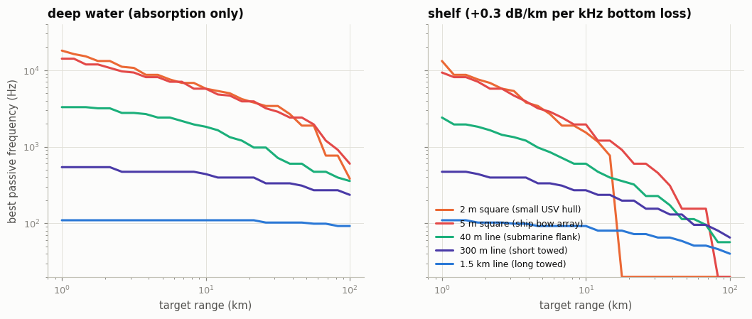
Reading the plot. Two regimes appear:
- Coherence-limited apertures (long lines): gain grows only slowly once the array is longer than ~30 λ, so the best frequency sits near where $L \approx 30\lambda$ and falls slowly with range. A 40 m flank array is best at ~0.7–2.4 kHz (5–30 km, deep water); a 1.5 km towed array near 100 Hz in deep water, falling to 40–65 Hz at 30–100 km on a shelf.
- Small apertures (hull arrays): gain keeps growing with frequency until absorption and bottom loss stop it. A 5 m bow array is best at ~3–7 kHz in deep water out to 30 km (~600 Hz at 100 km) and ~0.5–3 kHz on a shelf. A 2 m array on a small hull wants ~6–9 kHz at 5–10 km. On a shelf beyond ~15–60 km the small arrays' curves drop to the bottom of the plot: bottom loss eats all the gain they could add, so at long range they are no better than one hydrophone at low frequency.
Treat these numbers as illustrative. The last printed lines show how strongly they depend on the assumed slope $s$: for the 1.5 km line the best frequency moves from a few hundred Hz ($s$ = 0) to a few tens of Hz ($s$ = −2), and the frequency-proportional bottom loss is unphysical near modal cutoff. The model also leaves out tonals (which favour low frequency for passive detection and classification), the platform's flow noise (which falls with frequency and favours higher frequency on a moving hull), and the thermocline, which §3 adds. What is robust is the structure: small apertures are pushed up in frequency until absorption and bottom loss stop them; long apertures are capped by coherence and gain nothing from going higher.
3. The thermocline, mapped
The PE model (split-step Fourier; against the normal-mode solution for a 200 Hz shelf: bias 0.3 dB, rms 0.6 dB, and converged in range step) computes transmission loss for two environments with the same kind of mixed layer:
- deep water: 5 km deep, a 60 m mixed layer at 18 °C over a main thermocline, sound-channel axis near 1 km;
- shelf: 150 m deep, the 40 m mixed layer and thermocline of the FDTD runs in notebook 03.
Sources are a surface ship (5 m) and a submarine below the layer (150 m in deep water, 90 m on the shelf). The duct's cutoff frequency (Urick's rule) decides which frequencies it traps:
Code
for H in [20, 40, 60, 100]:
    print(f"mixed layer {H:3d} m: trapped above ~{pe.duct_cutoff_hz(H):5.0f} Hz")
mixed layer 20 m: trapped above ~ 1089 Hz mixed layer 40 m: trapped above ~ 385 Hz mixed layer 60 m: trapped above ~ 210 Hz mixed layer 100 m: trapped above ~ 97 Hz
Code
def tl_window(name, zr, r1_km, r2_km):
    d = cases.load_pe(name)
    r = d['r'] / 1000; z = d['z']; tl = d['tl'].astype(float)
    i = int(np.argmin(np.abs(z - zr))); sel = (r >= r1_km) & (r <= r2_km)
    return -10 * np.log10(np.mean(10 ** (-tl[i, sel] / 10)))       # incoherent average over the window

FREQS = [('100hz', '100 Hz'), ('1khz', '1 kHz'), ('3k5hz', '3.5 kHz')]
fig, axs = plt.subplots(2, 3, figsize=(12, 6.2), sharex=True, sharey=True)
for row, who in zip(axs, ['ship', 'sub']):
    for ax, (tag, flab) in zip(row, FREQS):
        d = cases.load_pe(f'pe_deep_{tag}_{who}')
        r = d['r'] / 1000; z = d['z']; top = z <= 400; sel = r <= 40
        im = ax.pcolormesh(r[sel], z[top], d['tl'].astype(float)[top][:, sel], cmap=style.SEQ.reversed(),
                           vmin=60, vmax=110, shading='auto', rasterized=True)
        ax.axhline(60, color=style.SURFACE, lw=0.8, ls=(0, (3, 3)))
        ax.plot([0], [float(d['zs'])], marker='*', color=style.ORANGE, ms=11, mec=style.INK, clip_on=False)
        ax.set_title(f"{flab}, {'surface ship (5 m)' if who == 'ship' else 'submarine (150 m)'}", loc='left', fontsize=9.5)
        ax.grid(False)
for ax in axs[:, 0]: ax.set_ylabel('depth (m)')
for ax in axs[1]: ax.set_xlabel('range (km)')
axs[0, 0].set_ylim(400, 0)
cb = fig.colorbar(im, ax=axs, shrink=0.8, pad=0.015); cb.set_label('transmission loss (dB); darker = louder')
fig.suptitle('Deep water, top 400 m: the 60 m mixed layer (dotted) traps sound above ~210 Hz', x=0.02, ha='left', fontsize=11)
style.save(fig, 'd_layer_deep_maps')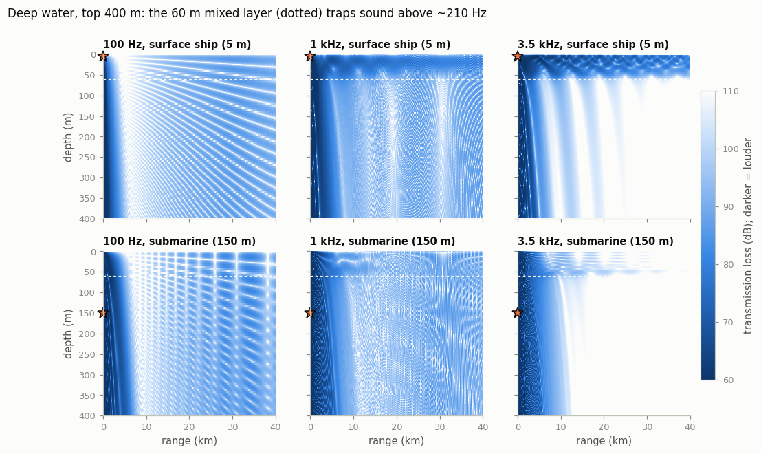
Code
d = cases.load_pe('pe_deep_1khz_ship')
fig, ax = plt.subplots(figsize=(11, 3.6))
im = ax.pcolormesh(d['r'] / 1000, d['z'], d['tl'].astype(float), cmap=style.SEQ.reversed(), vmin=60, vmax=110,
                   shading='auto', rasterized=True)
ax.set_ylim(5000, 0); ax.set_xlabel('range (km)'); ax.set_ylabel('depth (m)'); ax.grid(False)
ax.set_title('Deep water, 1 kHz, surface ship: surface duct, shadow zone, bottom bounce and a convergence zone near 55 km', loc='left')
cb = fig.colorbar(im, ax=ax, pad=0.01); cb.set_label('TL (dB)')
style.save(fig, 'd_deep_full_1khz')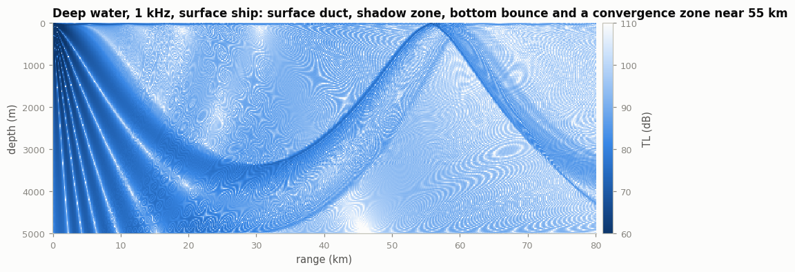
The maps show the regimes directly:
- 100 Hz is below the duct cutoff: the layer barely exists for it. Sound refracts downward from either source, and near-surface receivers see a deep shadow beyond a few km (made worse by the surface's Lloyd's mirror, which cancels low-angle sound near the surface at low frequency). Energy returns by bottom bounce and at the convergence zone (~55 km).
- 1 kHz and 3.5 kHz: the ship's sound is trapped in the duct and stays loud near the surface; the submarine's sound refracts down and away, and only leaks into the duct weakly.
The table puts numbers on it: incoherent average TL over 8–12 km and 25–35 km for a receiver in the layer (hull depth, 10 m), one just below it (150 m in deep water; 90 m on the shelf), and the best receiver depth for the submarine. The 3.5 kHz deep-water run is truncated at 1500 m (no bottom return; the convergence zone is beyond its 40 km). Near the surface at 100 Hz, TL overstates the SNR loss because ambient noise drops there too (notebook 07, §5).
Code
def best_depth(name, r1_km, r2_km, zmax):
    d = cases.load_pe(name)
    r = d['r'] / 1000; z = d['z']; sel = (r >= r1_km) & (r <= r2_km); ok = (z >= 5) & (z <= zmax)
    t = -10 * np.log10(np.mean(10 ** (-d['tl'].astype(float)[:, sel] / 10), axis=1))
    i = np.argmin(np.where(ok, t, np.inf)); return t[i], z[i]

rows = []
for water, zlow, zmax in [('deep', 150.0, 4900.0), ('shelf', 90.0, 145.0)]:
    for tag, flab in FREQS:
        for (r1, r2) in [(8, 12), (25, 35)]:
            if water == 'shelf' and r1 > 15: continue
            t = {(who, zr): tl_window(f'pe_{water}_{tag}_{who}', zr, r1, r2) for who in ['ship', 'sub'] for zr in [10.0, zlow]}
            # the 3.5 kHz deep run is truncated (absorbing) below 1500 m
            bt, bz = best_depth(f'pe_{water}_{tag}_sub', r1, r2, zmax if not (water == 'deep' and tag == '3k5hz') else 1400.0)
            rows.append((water, flab, f'{r1}-{r2} km', t[('ship', 10.0)], t[('ship', zlow)], t[('sub', 10.0)], t[('sub', zlow)], bt, bz))
print('Transmission loss (dB), incoherent average over the range window. Deep: "below" = 150 m; shelf: 90 m.')
print(f"{'water':6s} {'freq':8s} {'range':9s} | ship->10 m  ship->below | sub->10 m  sub->below  sub->best depth | sub penalty at 10 m")
for w, fl, rg, a, b_, c, dd, bt, bz in rows:
    print(f"{w:6s} {fl:8s} {rg:9s} | {a:8.1f}  {b_:10.1f}  | {c:8.1f}  {dd:9.1f}   {bt:6.1f} at {bz:4.0f} m | {c - a:+6.1f} dB")
Transmission loss (dB), incoherent average over the range window. Deep: "below" = 150 m; shelf: 90 m. water freq range | ship->10 m ship->below | sub->10 m sub->below sub->best depth | sub penalty at 10 m deep 100 Hz 8-12 km | 109.5 102.7 | 112.9 104.2 74.7 at 1704 m | +3.4 dB deep 100 Hz 25-35 km | 86.5 89.3 | 85.0 85.8 77.5 at 3122 m | -1.5 dB deep 1 kHz 8-12 km | 75.0 91.1 | 87.0 94.6 75.2 at 1644 m | +12.0 dB deep 1 kHz 25-35 km | 81.3 93.3 | 90.0 88.2 78.0 at 3033 m | +8.7 dB deep 3.5 kHz 8-12 km | 67.3 97.9 | 93.3 97.2 77.6 at 1369 m | +26.0 dB deep 3.5 kHz 25-35 km | 76.4 113.9 | 110.2 125.2 105.3 at 48 m | +33.8 dB shelf 100 Hz 8-12 km | 79.1 80.2 | 74.6 64.6 64.6 at 91 m | -4.4 dB shelf 1 kHz 8-12 km | 66.7 71.8 | 71.6 63.4 63.4 at 90 m | +4.9 dB shelf 3.5 kHz 8-12 km | 65.7 73.2 | 73.0 64.5 64.5 at 90 m | +7.4 dB
What the numbers say about the layer:
- The last column is the practical question for a hull sonar in the layer: how much harder is a submarine below the layer to hear than a surface source at the same range and source level? In deep water it is about 9–12 dB at 1 kHz and 26–34 dB at 3.5 kHz: the duct keeps the ship loud and the submarine's sound refracts deep. The effect grows with frequency because the duct traps higher frequencies more tightly. (The 34 dB at 25–35 km is an upper bound: that run has no bottom-bounce return.) This is the classic "below the layer" effect, and in deep water at mid frequency it is large.
- Putting a receiver just below the layer does not fix it in deep water: at 10 km the 150 m receiver is itself in the downward-refracted shadow. At 8–12 km the submarine's sound is loudest at 1.4–1.7 km depth, ~12–16 dB louder than at hull depth at 1–3.5 kHz (and ~38 dB at 100 Hz, where the near-surface shadow is deepest); at 25–35 km the best depth is ~3 km. The best depth moves with range, which is the case for deep vertical aperture, a variable-depth sensor, or a deep fixed receiver.
- At 100 Hz the layer is transparent (below the ~210 Hz duct cutoff). Near-surface receivers suffer instead from the Lloyd's mirror and the deep-water shadow zone, for both sources, until bottom bounce and the convergence zone return the energy.
- On the shelf the seabed returns sound through the whole column, and the layer's effect shrinks to ~5–7 dB at 1–3.5 kHz. At 100 Hz the submarine is actually the louder of the two at hull depth, because a source 5 m below a pressure-release surface radiates poorly at low frequency. For a submarine on the shelf the best receiver depth is close to its own depth, 8–10 dB better than 10 m. The FDTD run in notebook 03 (100 Hz, 3.5 km) found a 30 m receiver 7 dB below the best depth, consistent with this.
These are single environments; the size of the effect varies with the layer's depth and strength, sea state (surface roughness leaks the duct), the seabed and the season.
4. Rigid (hull) arrays, and an ideal-design sketch
What makes a good rigid array:
- Aperture in both dimensions (cylindrical, spherical or conformal): azimuth and elevation, no left/right ambiguity, vertical rejection of surface noise, some depth information.
- Design frequency set by aperture: about 10–30 λ across, elements at λ/2 at the top of the band. Hull size is what pushes hull sonar up to 1–5 kHz, exactly where submarines are quietest and the layer bites hardest (§3), which is why navies also tow arrays below the layer.
- Self noise usually decides performance: flow noise grows roughly 15–18 dB per doubling of speed and machinery noise travels through the hull. Arrays forward and away from machinery, decoupling mounts, baffles and acoustic windows, and "sprint and drift" operation.
- Processing: adaptive beamforming to null own-ship noise and loud contacts; long narrowband integration on tonals; vector sensors (pressure plus particle motion) so each element has directivity and small arrays resolve left from right.
- Passive ranging needs baselines: a rigid array focuses in range only within $L^2/\lambda$ (about 200 m for a 10 m array at 3 kHz), so hull sonar ranges passively only with widely separated sub-arrays, over a few km at most.
If the goal is maximum sensitivity and range:
| Fixed surveillance node | Ship or submarine | Small USV | |
|---|---|---|---|
| Band | 50–500 Hz passive | bow 0.5–5 kHz passive, ~3–4 kHz active; flank 0.2–2 kHz; towed < 500 Hz | hull array ~5–10 kHz (short range); low frequency only with dipped or towed lines |
| Aperture | horizontal 30–100 λ (300 m–1 km at 150 Hz) plus vertical through the channel or at depth | bow 5–8 m; flank 30–60 m; towed 1–2 km | 1–2 m on the hull; 100–150 m vertical line dipped |
| Placement | deep: sound-channel axis or the bottom (reliable acoustic path); shelf: full-column vertical lines | arrays forward, decoupled; tow below the layer | line below the surface-noise zone, heave-decoupled |
| Self noise | none (cabled, fixed) | the limiting factor; slow for passive search | propulsion off or electric; decoupled lines |
| Processing | adaptive, minutes-long narrowband, matched-field | adaptive, focused, tonal + broadband | coherent across the formation (notebook 07) |
In one line: size the aperture to one to a few coherence lengths at a frequency where absorption and bottom loss over the target range are a few dB, then spend the rest of the budget on quietness, vertical aperture and adaptive processing.
07 · Can a formation of USVs beat a towed array at 100 Hz?
For the multi-USV array, is there a system design where we could do better than a towed array by position controlling, say, 10 USVs at around 0.5 wavelengths and targeting around 100 Hz?
At 100 Hz the wavelength is 15 m, so half-wavelength spacing puts 10 USVs 7.5 m apart. This notebook compares that formation, and variations on it, with towed arrays, in the same shallow-water model used in notebooks 03 and 04:
- waveguide: 150 m of water over a sand-like bottom (Pekeris), 9 propagating modes at 100 Hz;
- noise: wind and distant shipping in equal parts (normal-mode noise), plus optional white self noise;
- signal: a submarine at 90 m or a surface ship at 5 m, 5–15 km away, with horizontal coherence $e^{-d/L_c}$, $L_c$ = 30 λ = 450 m (Carey);
- metric: output SNR relative to one quiet hydrophone at 30 m, so an array that puts its hydrophones in a poor place, or adds self noise, is charged for it;
- processing: matched-field weights (the modelled field of the true waveguide, source depth and range: an upper bound that needs a good environment model), or processing that needs no environment model: geometric focusing on the source point with free-space delays, or conventional plane-wave beams (the better of the two is shown).
Position and clocks are assumed known, as in the rest of the report; §4 asks how well they must be known.
Code
import sys, os
sys.path.insert(0, os.path.abspath('..'))
import numpy, scipy, matplotlib, PIL  # named here so the in-browser (JupyterLite) kernel loads them
import numpy as np
import matplotlib.pyplot as plt
from sonarsim import style, physics, arrays, modes, cases, formation as fm
style.use()
Code
# Parameters
F_HZ = 100.0
WATER_DEPTH = 150.0
LC_LAMBDA = 30             # horizontal coherence length in wavelengths
WIND, SHIPPING = 1.0, 1.0  # noise mix (relative powers)
SUB_DEPTH, SHIP_DEPTH = 90.0, 5.0
N_USV = 10

lam = 1500 / F_HZ
Lc = LC_LAMBDA * lam
wg = modes.Pekeris(F_HZ, WATER_DEPTH)
TOWED = arrays.towed_line(1500, arrays.half_wave_count(1500, F_HZ), 30)
TOWED_SHORT = arrays.towed_line(300, arrays.half_wave_count(300, F_HZ), 30)
VLA_DEPTHS = np.arange(5, WATER_DEPTH, lam / 2)      # a dipped line spanning the column at lambda/2

def gain(pos, zs=SUB_DEPTH, **kw):
    kw.setdefault('Lh', Lc); kw.setdefault('wind', WIND); kw.setdefault('shipping', SHIPPING)
    return fm.output_gain_db(wg, pos, zs, **kw)

G_TOWED = gain(TOWED)
print(f"{wg.nmodes} modes at {F_HZ:g} Hz; lambda = {lam:g} m; Lc = {Lc:g} m")
print(f"1.5 km towed array ({len(TOWED)} hydrophones, focused): {G_TOWED:.1f} dB;  300 m towed ({len(TOWED_SHORT)}): {gain(TOWED_SHORT):.1f} dB")
print(f"{len(VLA_DEPTHS)}-element dipped line: {VLA_DEPTHS[0]:g}-{VLA_DEPTHS[-1]:g} m")
9 modes at 100 Hz; lambda = 15 m; Lc = 450 m 1.5 km towed array (201 hydrophones, focused): 21.1 dB; 300 m towed (41): 17.0 dB 20-element dipped line: 5-147.5 m
1. Ten single hydrophones: spacing buys resolution, not gain
Each USV hangs one hydrophone at 30 m. The plot sweeps the spacing of a straight line of 10.
Code
spacings = np.array([2, 3, 5, 7.5, 10, 15, 22.5, 30, 45, 60, 90, 135, 200])
g_line = [gain(fm.dipped_array(fm.usv_positions(N_USV, s), [30.0])) for s in spacings]
fig, ax = plt.subplots(figsize=(7.6, 4.0))
ax.semilogx(spacings / lam, g_line, 'o-', color=style.ORANGE, ms=6, mec=style.SURFACE)
style.label_end(ax, spacings[-1] / lam, g_line[-1], f'{N_USV} USVs, one hydrophone each', style.ORANGE)
for g_, lab in [(G_TOWED, '1.5 km towed array'), (gain(TOWED_SHORT), '300 m towed array')]:
    ax.axhline(g_, color=style.BLUE, lw=1.5, ls=(0, (4, 3)))
    ax.text(spacings[0] / lam * 1.05, g_ + 0.4, lab, fontsize=8.5, color=style.INK2)
ax.axhline(10 * np.log10(N_USV), color=style.MUTED, lw=1)
ax.text(spacings[0] / lam * 1.05, 10 * np.log10(N_USV) - 1.1, f'10 log {N_USV}', fontsize=8.5, color=style.INK2)
ax.axvline(0.5, color=style.MUTED, lw=1, ls=(0, (2, 2)))
ax.set_xlabel('USV spacing (wavelengths)'); ax.set_ylabel('gain over one 30 m hydrophone (dB)')
ax.set_ylim(0, 25); ax.set_title(f'{N_USV} single hydrophones in a line at {F_HZ:g} Hz', loc='left')
style.save(fig, 'q4_usv_spacing')
i = int(np.argmax(g_line))
print(f"best spacing {spacings[i]:g} m ({spacings[i]/lam:.2f} lambda): {g_line[i]:.1f} dB;  at 45 m: {g_line[list(spacings).index(45)]:.1f} dB")
best spacing 10 m (0.67 lambda): 12.4 dB; at 45 m: 8.4 dB
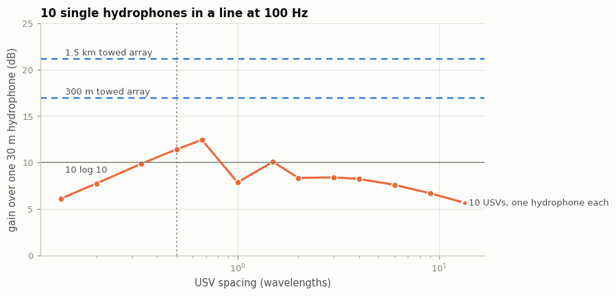
Half to two-thirds of a wavelength is in fact the best spacing for ten single hydrophones (11–12 dB): the shallow-water noise arrives near the horizontal, and at that spacing it is slightly anti-correlated between neighbours, so the array does a little better than $10\log_{10}10$. Spreading the USVs out narrows the beam but lets horizontal noise in through grating lobes (the dip at one wavelength) and, beyond a few hundred metres, loses signal coherence. Either way the formation stays between about 6 and 12 dB, roughly 10 dB short of a 1.5 km towed array. The spacing is not the problem; the number of coherent hydrophones is. A 10-USV line at λ/2 is a 70 m array, the length of a TB-16-class tactical towed array.
2. More hydrophones per USV: dipped vertical lines
Each USV lowers a vertical line of hydrophones at λ/2 (7.5 m) through the water column, so 10 USVs carry 200 hydrophones, the same as the 1.5 km towed array. The lines are spaced tens of metres apart (the formation no longer needs λ/2 horizontally; the vertical lines supply the element count).
Code
DESIGNS = [
    ('towed 1.5 km', TOWED, style.BLUE),
    ('towed 300 m', TOWED_SHORT, style.BLUE),
    (f'{N_USV} USVs, line at λ/2, 1 hydrophone', fm.dipped_array(fm.usv_positions(N_USV, lam / 2), [30.0]), style.ORANGE),
    (f'{N_USV} USVs, 190 m ring, 1 hydrophone', fm.dipped_array(fm.usv_positions(N_USV, 60, 'ring'), [30.0]), style.ORANGE),
    (f'{N_USV} USVs, line 45 m apart, dipped lines', fm.dipped_array(fm.usv_positions(N_USV, 45), VLA_DEPTHS), style.YELLOW),
    (f'{N_USV} USVs, 190 m ring, dipped lines', fm.dipped_array(fm.usv_positions(N_USV, 60, 'ring'), VLA_DEPTHS), style.YELLOW),
    (f'{2*N_USV} USVs, 380 m ring, dipped lines', fm.dipped_array(fm.usv_positions(2 * N_USV, 60, 'ring'), VLA_DEPTHS), style.YELLOW),
]
def robust(pos, zs, **kw):          # no environment model: better of geometric focus and plane-wave beams
    return max(gain(pos, zs, method='focus', **kw), gain(pos, zs, method='beam', **kw))

table = []
for lab, pos, col in DESIGNS:
    row = [v for zs in (SUB_DEPTH, SHIP_DEPTH) for v in (gain(pos, zs, method='matched'), robust(pos, zs))]
    table.append(row)
    print(f"{lab:42s} {len(pos):4d} hyd.  submarine: matched {row[0]:5.1f}  no-model {row[1]:5.1f}   "
          f"surface ship: matched {row[2]:5.1f}  no-model {row[3]:5.1f}")
table = np.array(table)
print(f"towed 1.5 km at 60 / 90 m: {robust(arrays.towed_line(1500, len(TOWED), 60), SUB_DEPTH):.1f} / "
      f"{robust(arrays.towed_line(1500, len(TOWED), 90), SUB_DEPTH):.1f} dB;  "
      f"target 10 deg off endfire: {robust(TOWED, SUB_DEPTH, bearing_deg=10):.1f} dB")

fig, axs = plt.subplots(1, 2, figsize=(11.5, 4.2), sharey=True)
yy = np.arange(len(DESIGNS))[::-1]
for ax, j, ttl in [(axs[0], 0, f'submarine, {SUB_DEPTH:g} m'), (axs[1], 2, f'surface ship, {SHIP_DEPTH:g} m')]:
    for y, (lab, pos, col), row in zip(yy, DESIGNS, table):
        ax.plot([row[j + 1], row[j]], [y, y], color=col, lw=2, alpha=0.5)
        ax.plot(row[j], y, 'o', color=col, ms=8, mec=style.SURFACE, label='matched-field (environment known)' if y == yy[0] else None)
        ax.plot(row[j + 1], y, 'o', mfc=style.SURFACE, mec=col, mew=1.8, ms=7, label='no environment model' if y == yy[0] else None)
    ax.axvline(table[0, j], color=style.BLUE, lw=1, ls=(0, (4, 3)))
    ax.set_title(ttl, loc='left'); ax.set_xlabel('gain over one 30 m hydrophone (dB)'); ax.set_xlim(0, 25)
axs[0].set_yticks(yy); axs[0].set_yticklabels([f'{d[0]} ({len(d[1])})' for d in DESIGNS], fontsize=8.5)
axs[0].legend(loc='upper left', fontsize=8)
style.save(fig, 'q4_usv_designs')
towed 1.5 km 201 hyd. submarine: matched 21.1 no-model 21.0 surface ship: matched 21.1 no-model 20.7 towed 300 m 41 hyd. submarine: matched 17.0 no-model 17.0 surface ship: matched 16.9 no-model 16.9 10 USVs, line at λ/2, 1 hydrophone 10 hyd. submarine: matched 11.4 no-model 11.4 surface ship: matched 11.4 no-model 11.4 10 USVs, 190 m ring, 1 hydrophone 10 hyd. submarine: matched 8.9 no-model 8.2 surface ship: matched 9.5 no-model 8.6 10 USVs, line 45 m apart, dipped lines 200 hyd. submarine: matched 17.4 no-model 12.5 surface ship: matched 19.4 no-model 15.9 10 USVs, 190 m ring, dipped lines 200 hyd. submarine: matched 18.0 no-model 13.3 surface ship: matched 18.6 no-model 14.4 20 USVs, 380 m ring, dipped lines 400 hyd. submarine: matched 19.9 no-model 14.5 surface ship: matched 20.2 no-model 14.1 towed 1.5 km at 60 / 90 m: 21.9 / 23.4 dB; target 10 deg off endfire: 13.4 dB
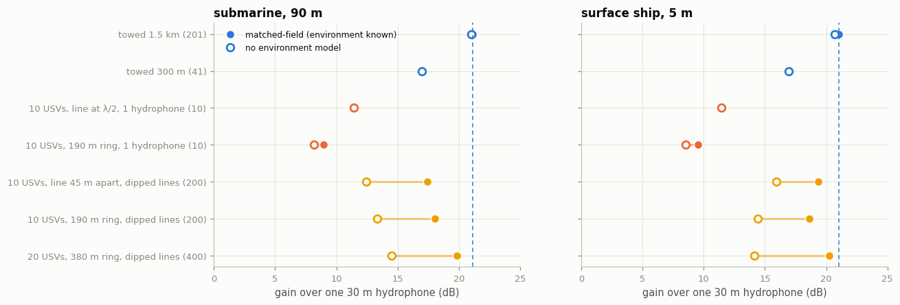
With 200 hydrophones on dipped lines, ten USVs come 3–4 dB short of the 1.5 km towed array for the submarine and ~2 dB short for the surface ship, and only with matched-field processing; twenty USVs (400 hydrophones) come within about 1 dB. Without an environment model the dipped lines lose 4–6 dB, because the modal field is not a plane wave (or a spherical wave) in the vertical. The towed array does not have this dependence: at 100 Hz a 1.5 km array is in its own near field out to $L^2/\lambda$ = 150 km, but simple geometric focusing recovers its full gain.
The towed baseline here is at 30 m and broadside, its best bearing. Lowered to 60–90 m it gains another 1–2 dB against this submarine; 10° off endfire it loses ~8 dB, where a ring formation does not.
So, on ambient noise alone and at equal hydrophone count, the formation does not beat a long towed array; it reaches parity only with twice the hydrophones and a good environment model. The balance can shift through self noise.
3. Self noise decides it
A towed array at a few knots adds flow and platform noise, typically several dB above ambient at low frequency. A USV formation can drift or hold station slowly with propulsion off or on quiet electric thrusters; its hydrophones still pick up cable strum, heave and wave slap unless the lines are decoupled. The plot adds white self noise to each design (relative to the ambient level per hydrophone) against a quiet reference hydrophone.
Code
# Parameters
SELF_NOISE_DB = np.arange(-10, 11, 2.0)
USV_DESIGN = DESIGNS[5]          # 10 USVs on a ring with dipped lines

sn_t = [gain(TOWED, self_noise_db=s) for s in SELF_NOISE_DB]
sn_u = [gain(USV_DESIGN[1], self_noise_db=s) for s in SELF_NOISE_DB]
fig, ax = plt.subplots(figsize=(7.6, 4.0))
ax.plot(SELF_NOISE_DB, sn_t, color=style.BLUE); style.label_end(ax, SELF_NOISE_DB[-1], sn_t[-1], 'towed 1.5 km', style.BLUE)
ax.plot(SELF_NOISE_DB, sn_u, color=style.YELLOW); style.label_end(ax, SELF_NOISE_DB[-1], sn_u[-1], USV_DESIGN[0], style.YELLOW)
ax.set_xlabel('self noise per hydrophone relative to ambient (dB)'); ax.set_ylabel('gain over a quiet 30 m hydrophone (dB)')
ax.set_title('Effect of platform self noise (submarine target, matched processing)', loc='left')
ax.set_ylim(5, 25)
style.save(fig, 'q4_usv_self_noise')
for st, su in [(3, -10), (6, -10), (6, 0), (0, 0)]:
    print(f"towed self noise {st:+d} dB vs USV {su:+d} dB: towed {gain(TOWED, self_noise_db=st):.1f} dB, "
          f"USVs {gain(USV_DESIGN[1], self_noise_db=su):.1f} dB matched-field, {robust(USV_DESIGN[1], SUB_DEPTH, self_noise_db=su):.1f} dB without a model")
towed self noise +3 dB vs USV -10 dB: towed 15.1 dB, USVs 17.9 dB matched-field, 13.2 dB without a model towed self noise +6 dB vs USV -10 dB: towed 12.7 dB, USVs 17.9 dB matched-field, 13.2 dB without a model towed self noise +6 dB vs USV +0 dB: towed 12.7 dB, USVs 16.7 dB matched-field, 12.0 dB without a model towed self noise +0 dB vs USV +0 dB: towed 17.1 dB, USVs 16.7 dB matched-field, 12.0 dB without a model
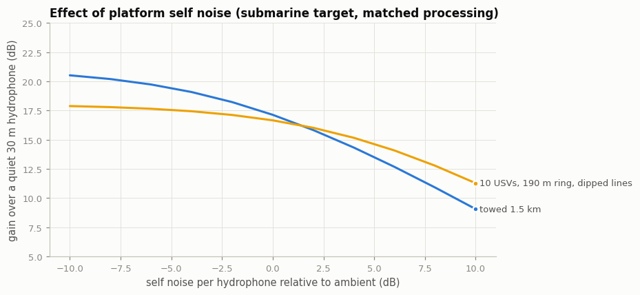
The plot gives both designs the same self noise. A towed array is hurt more by it than the formation is, because much of its advantage came from rejecting the structured, near-horizontal ambient noise; once uncorrelated flow noise dominates, that advantage goes, and the curves cross at about 1–2 dB above ambient. The printed cases give each platform its own level: with the towed array 3–6 dB above ambient and quiet USVs (10 dB below ambient), the formation leads by roughly 3–5 dB with matched-field processing, but only draws level (−2 to +0.5 dB) without it; with both at ambient level the two are within half a decibel.
Two caveats weigh on this. The USV self noise is modelled as white; real strum, heave and vehicle noise are correlated along a line and strongest in the top elements, so −10 dB is an optimistic design target, not a given. And part of the towed array's larger loss is that it rejected the structured ambient noise better in the first place. Quiet vehicles, decoupled lines and a good environment model are therefore the design drivers, more than the geometry.
4. Position control versus position knowledge
Coherent processing needs each hydrophone's position to a fraction of a wavelength, but the positions need to be known, not held. The formation can wander by metres as long as the beamformer uses measured positions. The plot adds random, unknown 3D errors to every hydrophone.
Code
# Parameters
POS_ERR_M = [0, 0.5, 1, 1.5, 2, 3, 4, 6]
TRIALS = 6

r_sub = np.linspace(5000, 15000, 11)
pe_g = [gain(USV_DESIGN[1], pos_error_m=s, n_trials=TRIALS, ranges_m=r_sub) for s in POS_ERR_M]
# correlated error: each line tilted by an unknown angle in a random direction (current drag)
rng = np.random.default_rng(1)
base = USV_DESIGN[1]; n_el = len(VLA_DEPTHS)
for tilt in [1, 2, 5]:
    tp = base.copy()
    for i in range(len(base) // n_el):
        a = rng.uniform(0, 2 * np.pi); sl = slice(i * n_el, (i + 1) * n_el)
        off = np.tan(np.radians(tilt)) * (base[sl, 2] - base[sl, 2].min())
        tp[sl, 0] += off * np.cos(a); tp[sl, 1] += off * np.sin(a)
    print(f"unknown line tilt {tilt} deg (bottom offset {np.tan(np.radians(tilt))*(VLA_DEPTHS[-1]-VLA_DEPTHS[0]):.1f} m): "
          f"{gain(base, true_pos=tp) - gain(base):+.1f} dB")
fig, ax = plt.subplots(figsize=(7.0, 3.8))
ax.plot(POS_ERR_M, np.array(pe_g) - pe_g[0], 'o-', color=style.YELLOW, ms=6, mec=style.SURFACE)
ax.axvline(lam / 10, color=style.MUTED, lw=1, ls=(0, (2, 2))); ax.text(lam / 10 + 0.1, -9, 'λ/10', fontsize=8.5, color=style.INK2)
ax.set_xlabel('rms unknown position error per hydrophone (m)'); ax.set_ylabel('change in gain (dB)')
ax.set_ylim(-10, 0.5); ax.set_title(f'{USV_DESIGN[0]}: tolerance to position errors at {F_HZ:g} Hz', loc='left')
style.save(fig, 'q4_usv_position_error')
print(dict(zip(POS_ERR_M, np.round(np.array(pe_g) - pe_g[0], 1))))
unknown line tilt 1 deg (bottom offset 2.5 m): -0.5 dB
unknown line tilt 2 deg (bottom offset 5.0 m): -3.4 dB
unknown line tilt 5 deg (bottom offset 12.5 m): -8.9 dB
{0: np.float64(0.0), 0.5: np.float64(-0.1), 1: np.float64(-0.3), 1.5: np.float64(-0.6), 2: np.float64(-1.0), 3: np.float64(-2.2), 4: np.float64(-3.9), 6: np.float64(-8.8)}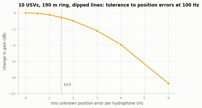
Random errors up to about 1 m (λ/15) cost almost nothing; 2 m costs ~1 dB; 4 m costs ~4 dB. Correlated errors are more dangerous: a 150 m line tilted by an unknown 2° (5 m offset at the bottom) costs ~3 dB, and 5° costs ~9 dB. The requirement is therefore ~1 m knowledge of every hydrophone, including each line's shape, not 1 m station-keeping. RTK GNSS gives the USVs to centimetres, but a hydrophone 100 m down a line moves with current and heave, so each line needs its own positioning (depth sensors plus an acoustic or inertial fix of the line shape). Clock synchronisation to ~1 ms (λ/10 at 100 Hz) is trivial with GNSS time.
5. Hydrophone depth under a USV
A hydrophone near the sea surface sits in the pressure-release node of every mode (the Lloyd's mirror effect). But ambient noise, which also arrives through the modes, drops there too, so ambient-limited SNR changes less than the signal level does:
Code
z = np.array([1, 2, 3, 5, 8, 12, 20, 30, 45, 60, 90, 120, 140])
fig, ax = plt.subplots(figsize=(5.2, 4.4))
for zs, col, lab in [(SUB_DEPTH, style.VIOLET, f'submarine, {SUB_DEPTH:g} m'), (SHIP_DEPTH, style.ORANGE, f'surface ship, {SHIP_DEPTH:g} m')]:
    s = fm.depth_snr_db(wg, z, zs, WIND, SHIPPING)
    ax.plot(s, z, 'o-', color=col, ms=4, label=lab)
ax.axvline(0, color=style.MUTED, lw=1)
ax.set_ylim(WATER_DEPTH, 0); ax.set_xlim(-8, 4)
ax.set_xlabel('ambient-limited SNR (dB re column average)'); ax.set_ylabel('hydrophone depth (m)')
ax.legend(loc='lower left', fontsize=8.5); ax.set_title(f'Single hydrophone at {F_HZ:g} Hz', loc='left')
style.save(fig, 'q4_usv_depth')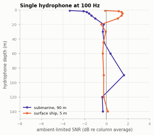
In ambient noise a hull-mounted hydrophone loses only a few dB at 100 Hz. The practical reason to go deeper is platform noise: wave slap, hull vibration, propulsion and heave-driven flow are all strongest at the surface. A hydrophone on a compliant (heave-isolated) suspension tens of metres down is the sonobuoy solution to this.
6. Geometry: bearing, ambiguity and range
Gain is not the only output. A straight line of USVs has the towed array's left/right ambiguity; a ring or an irregular 2D pattern does not, and a formation a few hundred metres across can focus in range as well as bearing out to a few km. The animations show both 10-USV geometries at 100 Hz (free-space, perfectly coherent: they show geometry, not detection).
Code
cases.show('plan_usv_line')Code
cases.show('plan_usv_ring')The half-wavelength line focuses to a broad bearing fan (~11° wide) with its mirror image. The 190 m ring puts a single, much tighter spot on the source with ~1/N sidelobes around it: bearing to a few degrees with no mirror, and some range information because the source is inside the ring's focusing distance ($D^2/\lambda$ ≈ 2.4 km).
7. What the gains mean for detection range
At 100 Hz absorption is negligible and spreading beyond the water depth is cylindrical (3 dB per doubling of range), so every 3 dB of gain roughly doubles detection range until bottom loss takes over. The table gives the range at which each design detects a target that the quiet 1.5 km towed array detects at 20 km (0.3 dB/km bottom loss).
Code
# Parameters
REF_RANGE_KM = 20.0
BOTTOM_LOSS_DB_KM = 0.3
TOWED_SELF_NOISE_DB = 0.0     # try 3-6
USV_SELF_NOISE_DB = -10.0

r = np.linspace(200, 200000, 20000)
tl = physics.transmission_loss(r, F_HZ, WATER_DEPTH, BOTTOM_LOSS_DB_KM)
g_ref = gain(TOWED, self_noise_db=TOWED_SELF_NOISE_DB if TOWED_SELF_NOISE_DB else None)
budget = np.interp(REF_RANGE_KM * 1000, r, tl) - g_ref       # SL - NL - DT for the reference target
print(f"{'design':44s} {'gain':>6s} {'range':>8s}")
for lab, pos, col in DESIGNS:
    sn = TOWED_SELF_NOISE_DB if lab.startswith('towed') else USV_SELF_NOISE_DB
    g_ = gain(pos, self_noise_db=sn if sn else None)
    rng_km = r[np.argmin(np.abs(tl - (budget + g_)))] / 1000
    print(f"{lab:44s} {g_:5.1f}  {rng_km:6.1f} km")
design gain range towed 1.5 km 21.1 20.0 km towed 300 m 17.0 12.7 km 10 USVs, line at λ/2, 1 hydrophone 10.8 5.2 km 10 USVs, 190 m ring, 1 hydrophone 8.5 3.5 km 10 USVs, line 45 m apart, dipped lines 17.3 13.2 km 10 USVs, 190 m ring, dipped lines 17.9 14.2 km 20 USVs, 380 m ring, dipped lines 19.7 17.3 km
Answer
Not with ten single hydrophones. Ten USVs at λ/2 form a 70 m array: about 11 dB of gain, close to the best (12.4 dB, at ~0.7 λ) any spacing of ten single hydrophones achieves, but roughly 10 dB less than a 1.5 km towed array. In the range model of §7 that is about a quarter of the detection range (5 km against 20 km). Position control does not change that; the number of coherent hydrophones does.
Possibly, with a different design and some favourable conditions. The version of the idea that competes is:
- Many hydrophones per vehicle: each USV lowers a vertical line at λ/2 through the water column (20 hydrophones over 150 m). Ten USVs then carry as many hydrophones as the towed array; twenty carry twice as many.
- Spacing set by coherence and geometry, not λ/2: vehicles tens of metres apart on a ring or irregular 2D pattern, a few hundred metres across (inside the ~450 m coherence length). This removes left/right ambiguity and gives some range from focusing, and no weak endfire direction.
- Quiet platforms: drifting or slow electric vehicles and heave-decoupled lines. Against a towed array with 3–6 dB of self noise, a formation 10 dB quieter than ambient is 3–5 dB ahead with matched-field processing.
- Matched-field processing with a surveyed environment model, to use the vertical lines' full gain (without a model they lose 4–6 dB of it, and the advantage in 3 disappears). Real mismatch costs part of this; it also gives source depth, so surface ships can be rejected (notebook 04).
- Hydrophone positions known to ~1 m, including each line's tilt and shape, from depth sensors and acoustic tracking; the vehicles only need to keep formation to within metres and avoid each other.
In this model, at equal hydrophone count and on ambient noise alone, the formation is 3–4 dB short of a quiet 1.5 km towed array; it pulls ahead only if its vehicles and lines are much quieter than the tow and the environment is well modelled. Its unconditional advantages are elsewhere: full-column coverage, depth classification, 360° coverage with no endfire weakness, and a 3D position fix. The main risks are practical: line strumming and heave noise, keeping 150 m lines near vertical in current and measuring their shape, and matched-field mismatch.
Model limits for this notebook: isovelocity Pekeris waveguide (no thermocline), perfect vertical coherence, azimuthally uniform shipping noise, white self noise, and no own-ship radiated noise for the tow.
05 · Animations and your own cases
Seven animations are pre-rendered (GIF here, MP4 in renders/). Each is defined in sonarsim/cases.py with every
parameter visible; copy one, change fields, and render it.
| Case | What it shows | Model |
|---|---|---|
plan_towed |
a 1.5 km towed array localises a 15 Hz transient to a bearing band, with its left/right mirror | coherent wave field, horizontal plane |
plan_distributed |
9 nodes 5 km apart focus the same transient to a ~50 m spot, assuming perfect coherence | same |
plan_distributed_jitter |
the same nodes with 40 m random path errors: coherent focusing breaks down | same |
section_surface_ship |
a 5 m source on a 150 m shelf with a thermocline, heard by a vertical array | 2D FDTD, range × depth |
section_sub_below_layer |
a 90 m source below the layer: energy concentrates deep; 30 m tow depth is 7 dB below the best depth, 2 dB below average | same |
plan_usv_line |
10 USVs at half-wavelength spacing, 100 Hz: a broad bearing fan and its mirror | coherent wave field, horizontal plane |
plan_usv_ring |
10 USVs on a 190 m ring, 100 Hz: a tight spot with no mirror | same |
The pe_* cases (notebook 06) are transmission-loss maps rather than movies; cases.render() saves them as .npz.
Code
import sys, os
sys.path.insert(0, os.path.abspath('..'))
import numpy, scipy, matplotlib, PIL  # named here so the in-browser (JupyterLite) kernel loads them
from sonarsim import cases
for name, c in cases.CASES.items():
    print(f"{name:26s} {c.title}")
plan_towed Towed array (1.5 km): a transient and its back-projection plan_distributed Distributed nodes (3 x 3, 5 km apart): same transient plan_distributed_jitter Distributed nodes, coherence lost (random 40 m path errors) plan_usv_line 10 USVs in a line, half a wavelength apart (100 Hz) plan_usv_ring 10 USVs on a 190 m ring (100 Hz) section_surface_ship Surface ship (5 m) - what a vertical array hears section_sub_below_layer Submarine below the layer (90 m) pe_deep_100hz_ship Deep water, 100 Hz, source at 5 m pe_shelf_100hz_ship 150 m shelf, 100 Hz, source at 5 m pe_deep_100hz_sub Deep water, 100 Hz, source at 150 m pe_shelf_100hz_sub 150 m shelf, 100 Hz, source at 90 m pe_deep_1khz_ship Deep water, 1000 Hz, source at 5 m pe_shelf_1khz_ship 150 m shelf, 1000 Hz, source at 5 m pe_deep_1khz_sub Deep water, 1000 Hz, source at 150 m pe_shelf_1khz_sub 150 m shelf, 1000 Hz, source at 90 m pe_deep_3k5hz_ship Deep water, 3500 Hz, source at 5 m pe_shelf_3k5hz_ship 150 m shelf, 3500 Hz, source at 5 m pe_deep_3k5hz_sub Deep water, 3500 Hz, source at 150 m pe_shelf_3k5hz_sub 150 m shelf, 3500 Hz, source at 90 m
Code
cases.show('plan_towed')Code
cases.show('plan_distributed')Code
cases.show('plan_distributed_jitter')Code
cases.show('section_surface_ship')Code
cases.show('section_sub_below_layer')Code
cases.show('plan_usv_line')Code
cases.show('plan_usv_ring')Make your own
Every case is a frozen dataclass; .replace(...) returns a modified copy. Plan-view cases are analytic and take
seconds (in the browser use quick=True). Section cases run the FDTD solver: about 2 minutes each with desktop
numpy; in the browser use quick=True for a coarse preview, or run the notebook locally for full quality.
Example 1: a ring of 6 nodes, 3 km radius, with small path errors. Change any field and re-run.
Code
# Parameters
my_plan = cases.get('plan_distributed').replace(
    name='my_ring',
    title='6 nodes on a 3 km ring, 15 m path errors',
    n_nodes=6, node_layout='ring', node_spacing_m=3000.0,
    timing_sigma_m=15.0,
    target_xy=(2000.0, -1500.0),
)
cases.render(my_plan, out_dir='../renders/custom', quick=True)
Example 2: a deeper submarine and a different thermocline. This one is slow in the browser; set RUN = True
to render it (use quick=True there).
Code
# Parameters
RUN = False
my_section = cases.get('section_sub_below_layer').replace(
    name='my_section',
    title='Submarine at 120 m, sharp layer at 30 m',
    source_depth_m=120.0, mixed_layer_m=30.0, thermocline_bottom_m=50.0,
    t_surface_c=22.0, t_below_c=8.0,
)
if RUN:
    display(cases.render(my_section, out_dir='../renders/custom', quick=True))
else:
    print('Set RUN = True to render', my_section.name)
Set RUN = True to render my_section
Fields you can change
PlanCase: layout ('towed', 'distributed', 'both'), towed_length_m, towed_center, towed_heading_deg,
n_nodes, node_spacing_m, node_layout ('grid', 'ring', 'random'), target_xy, extent_m, f0_hz,
timing_sigma_m, seed.
SectionCase: source_depth_m, source_range_m, f0_hz, cycles, range_m, depth_m, mixed_layer_m,
thermocline_bottom_m, t_surface_c, t_below_c, t_bottom_c, sediment_m, c_sed, rho_sed, vla_range_m,
vla_top_m, vla_bottom_m, vla_elements, tow_depth_m, t_end_s, ppw (grid points per wavelength), n_frames.
To regenerate every pre-rendered case after changing defaults: python scripts/render_cases.py.